目錄
@[toc]
前言
這次使用一個貓的數據集,我們使用深度神經網絡來識別這個是貓或者不是貓。

導包
這裏導入了兩個工具類,可以從這裏下載,這裏包含了這個函數和用到的數據集,其中用到了h5py,如果讀者沒有安裝的話,要先用pip安裝這個庫,還有以下用到的庫也要安裝。
# coding=utf-8
from dnn_utils_v2 import sigmoid, sigmoid_backward, relu, relu_backward
from lr_utils import load_dataset
import numpy as np
import matplotlib.pyplot as plt
import scipy
from scipy import ndimage
初始化網絡參數
在網絡定義之前,需要先對網絡的參數進行初始化,這裏分兩個來初始化,一個是兩層網絡的,另一個是L層網絡的。
兩層網絡的初始化
對兩層網絡的參數初始化要用到輸入層的大小、隱藏層的大小、輸出層的大小。
def initialize_parameters(n_x, n_h, n_y):
    """
    初始化參數
    :param n_x: 輸入層的大小。
    :param n_h: 隱藏層的大小。
    :param n_y: 輸出層的大小。
    :return:
     parameters -- 包含您的參數的python字典:
                    W1 -- 形狀重量矩陣(n_h, n_x)
                    b1 -- 形狀的偏置向量(n_h, 1)
                    W2 -- 形狀重量矩陣(n_y, n_h)
                    b2 -- 形狀的偏置向量(n_y, 1)
    """
    W1 = np.random.randn(n_h, n_x) * 0.01
    b1 = np.zeros((n_h, 1))
    W2 = np.random.randn(n_y, n_h) * 0.01
    b2 = np.zeros((n_y, 1))

    assert (W1.shape == (n_h, n_x))
    assert (b1.shape == (n_h, 1))
    assert (W2.shape == (n_y, n_h))
    assert (b2.shape == (n_y, 1))

    parameters = {"W1": W1,
                  "b1": b1,
                  "W2": W2,
                  "b2": b2}

    return parameters
L層網絡的初始化
對於更深的網絡,需要的參數是網絡中每一層的尺寸的python數組。相關的計算如下:
| | Shape of W | Shape of b | Activation | Shape of Activation
:—: | :—: | :—: | :—: | :—:
| Layer 1 | \((n^{[1]},12288)\) | \((n^{[1]},1)\) | $Z^{[1]} = W^{[1]} X + b^{[1]} $ | \((n^{[1]},209)\)
|Layer 2|\((n^{[2]}, n^{[1]})\)|\((n^{[2]},1)\)|\(Z^{[2]} = W^{[2]} A^{[1]} + b^{[2]}\)|\((n^{[2]}, 209)\)
|\(\vdots\)|\(\vdots\)|\(\vdots\)|\(\vdots\)|\(\vdots\)
|Layer L-1|\((n^{[L-1]}, n^{[L-2]})\)|\((n^{[L-1]}, 1)\)|\(Z^{[L-1]} = W^{[L-1]} A^{[L-2]} + b^{[L-1]}\)|\((n^{[L-1]}, 209)\)
|Layer L|\((n^{[L]}, n^{[L-1]})\)| \((n^{[L]}, 1)\)|\(Z^{[L]} = W^{[L]} A^{[L-1]} + b^{[L]}\)|\((n^{[L]}, 209)\)
def initialize_parameters_deep(layer_dims):
    """
    初始化深度參數
    :param layer_dims: 包含我們網絡中每一層的尺寸的python數組(列表)。
    :return:
     parameters -- python字典包含參數的"W1", "b1", ..., "WL", "bL":
                    Wl -- 形狀權重矩陣(layer_dims[l], layer_dims[l-1])
                    bl -- 形狀偏差向量(layer_dims[l], 1)
    """
    parameters = {}
    L = len(layer_dims)  # number of layers in the network

    for l in range(1, L):
        parameters['W' + str(l)] = np.random.randn(layer_dims[l], layer_dims[l - 1]) / np.sqrt(
            layer_dims[l - 1])  # *0.01
        parameters['b' + str(l)] = np.zeros((layer_dims[l], 1))

        assert (parameters['W' + str(l)].shape == (layer_dims[l], layer_dims[l - 1]))
        assert (parameters['b' + str(l)].shape == (layer_dims[l], 1))

    return parameters
正向傳播模塊
一個完整的神經網絡流程是如圖所示:
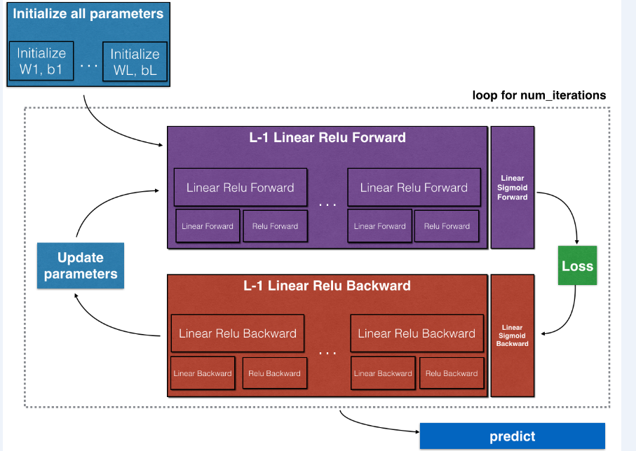
在這一部分,我們要完成的是紫色部分的正向傳播,其中包括線性正向傳播、線性激活正向傳播和完成整個正向傳播的L層模型正向傳播。
線性正向傳播
構建前向傳播的線性部分,使用的線性公式如下:
\(\(Z^{[l]} = W^{[l]}A^{[l-1]} +b^{[l]}\tag{1}\)\)
def linear_forward(A, W, b):
    """
    實現一個層的正向傳播的線性部分。
    :param A: 前一層(或輸入數據)的激活:(前一層的大小,示例的數量)
    :param W: 權重矩陣:形狀的numpy數組(當前層的大小,上一層的大小)
    :param b: 偏置向量,形狀的numpy數組(當前層的大小,1)
    :return:
    Z -- 激活函數的輸入,也稱爲預激活參數。
    cache -- :包含“a”、“W”和“b”的python字典;存儲用於有效地計算向後傳遞。
    """
    Z = np.dot(W, A) + b

    assert (Z.shape == (W.shape[0], A.shape[1]))
    cache = (A, W, b)

    return Z, cache
線性激活正向傳播
這裏使用到了兩個激活函數:
- Sigmoid:\(\sigma(Z) = \sigma(W A + b) = \frac{1}{ 1 + e^{-(W A + b)}}\)
- ReLU:\(A = ReLU(Z) = max(0, Z)\)
從線性到激活使用到的公式如下:
\(\(A^{[l]} = g(Z^{[l]}) = g(W^{[l]}A^{[l-1]} +b^{[l]})\tag{2}\)\)
def linear_activation_forward(A_prev, W, b, activation):
    """
    實現線性->激活層的正向傳播。
    :param A_prev: 前一層(或輸入數據)的激活:(前一層的大小,示例的數量)
    :param W: 權重矩陣:形狀的numpy數組(當前層的大小,上一層的大小)
    :param b: 偏置向量,形狀的numpy數組(當前層的大小,1)
    :param activation: 在此層中使用的激活,存儲爲文本字符串:“sigmoid”或“relu”
    :return:
     A -- 激活函數的輸出,也稱爲激活後值。
    cache --包含“線性緩存”和“activation_cache”的python字典;
             存儲用於有效地計算向後傳遞
    """
    if activation == "sigmoid":
        Z, linear_cache = linear_forward(A_prev, W, b)
        A, activation_cache = sigmoid(Z)

    elif activation == "relu":
        Z, linear_cache = linear_forward(A_prev, W, b)
        A, activation_cache = relu(Z)

    assert (A.shape == (W.shape[0], A_prev.shape[1]))
    cache = (linear_cache, activation_cache)

    return A, cache
L層模型正向傳播
根據線性正向傳播和線性激活正向傳播的循環L次,得到一個L層的模型,如下圖:
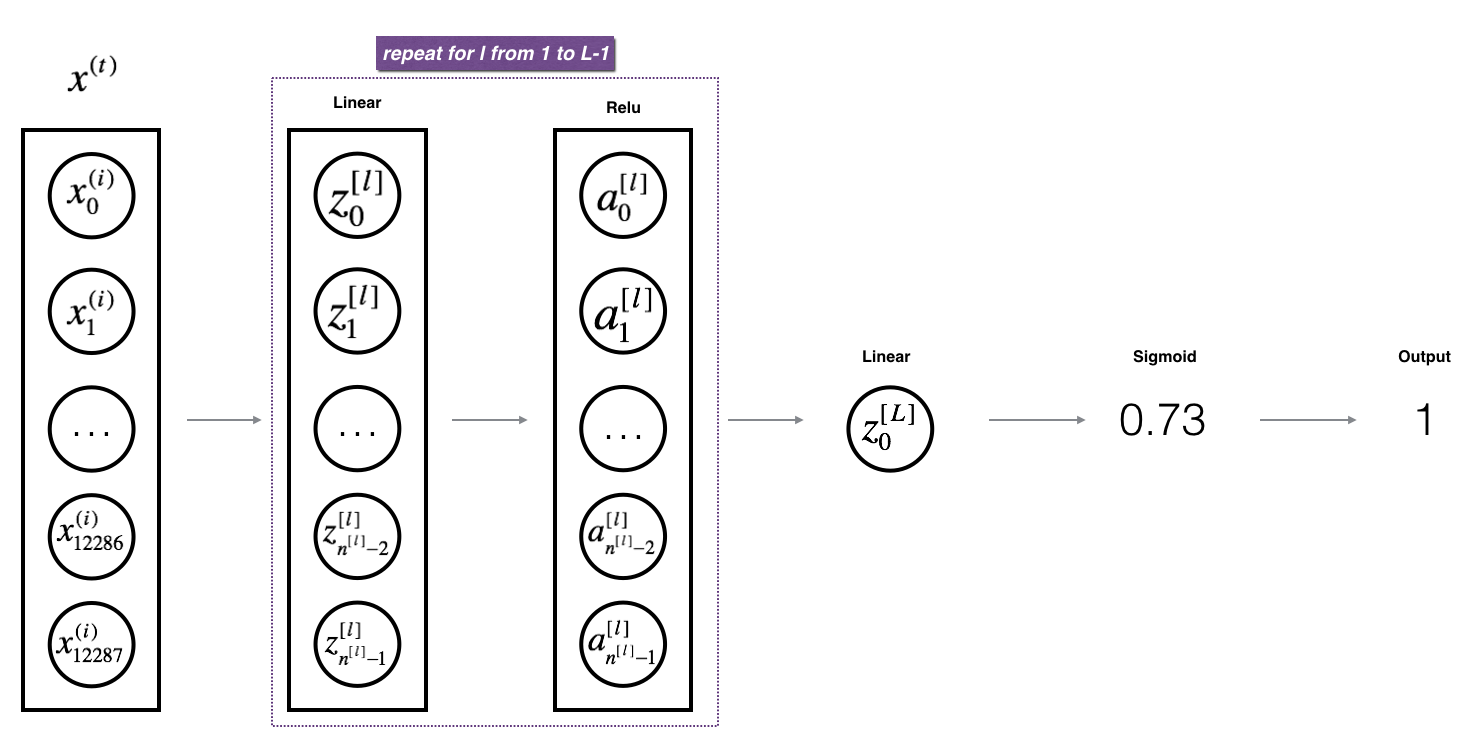
代碼中使用到的AL是指公式的\(A^{[L]}\):
\(\(A^{[L]} = \sigma(Z^{[L]}) = \sigma(W^{[L]} A^{[L-1]} + b^{[L]})\tag{3}\)\)
def L_model_forward(X, parameters):
    """
    爲[LINEAR->RELU]*(L-1)->LINEAR->SIGMOID計算實現正向傳播。
    :param X: 數據,形狀的numpy數組(輸入大小,示例數量)
    :param parameters: initialize_parameters_deep()的輸出
    :return:
    AL -- 最後激活後值
    caches -- 緩存包含列表:
                線性_activation_forward()的每個緩存(其中有L-1,從0到L-1的索引)
    """
    caches = []
    A = X
    L = len(parameters) // 2  # number of layers in the neural network

    # Implement [LINEAR -> RELU]*(L-1). Add "cache" to the "caches" list.
    for l in range(1, L):
        A_prev = A
        A, cache = linear_activation_forward(A_prev, parameters['W' + str(l)], parameters['b' + str(l)],
                                             activation="relu")
        caches.append(cache)

    # Implement LINEAR -> SIGMOID. Add "cache" to the "caches" list.
    AL, cache = linear_activation_forward(A, parameters['W' + str(L)], parameters['b' + str(L)], activation="sigmoid")
    caches.append(cache)

    assert (AL.shape == (1, X.shape[1]))

    return AL, caches
計算損失函數
計算成本函數的公式如下:
\(\(cost = -\frac{1}{m} \sum\limits_{i = 1}^{m} (y^{(i)}\log\left(a^{[L] (i)}\right) + (1-y^{(i)})\log\left(1- a^{[L](i)}\right)) \tag{4}\)\)
def compute_cost(AL, Y):
    """
    實現由公式(7)定義的成本函數。
    :param AL: 對應於你的標籤預測的概率向量,形狀(1,例子數)
    :param Y: 正確的“標籤”矢量(例如:如果非cat,則包含0)、形狀(1、示例數量)
    :return:
    cost -- 交叉熵損失
    """
    m = Y.shape[1]

    cost = -(np.sum(np.dot(Y, np.log(AL).T) + np.dot((1 - Y), np.log(1 - AL).T))) / m

    cost = np.squeeze(cost)
    assert (cost.shape == ())

    return cost
反向傳播模塊
就像向前傳播一樣,實現反向傳播的輔助函數。反向傳播用於計算損失函數與參數的梯度
線性反向傳播
在反向傳播的時候使用到公式如下:
$$ dW^{[l]} = \frac{\partial \mathcal{L} }{\partial W^{[l]}} = \frac{1}{m} dZ^{[l]} A^{[l-1] T} \tag{5}$$
$$ db^{[l]} = \frac{\partial \mathcal{L} }{\partial b^{[l]}} = \frac{1}{m} \sum_{i = 1}^{m} dZ^{l}\tag{6}$$
$$ dA^{[l-1]} = \frac{\partial \mathcal{L} }{\partial A^{[l-1]}} = W^{[l] T} dZ^{[l]} \tag{7}$$
def linear_backward(dZ, cache):
    """
    實現單層(l層)反向傳播的線性部分
    :param dZ: 線性輸出(當前層l)的成本梯度
    :param cache: 來自當前層的正向傳播元組(A_prev, W, b)的值
    :return:
    dA_prev -- 關於激活(前一層l-1)的成本梯度,與A_prev相同。
    dW -- 關於W(當前層l)的成本梯度,與W相同。
    db -- :b(當前層l)的成本梯度,與b相同。
    """
    A_prev, W, b = cache
    m = A_prev.shape[1]

    dW = np.dot(dZ, A_prev.T) / m
    db = np.sum(dZ, axis=1, keepdims=True) / m
    dA_prev = np.dot(W.T, dZ)

    assert (dA_prev.shape == A_prev.shape)
    assert (dW.shape == W.shape)
    assert (db.shape == b.shape)

    return dA_prev, dW, db
線性激活反向傳播
在這裏使用到的計算公式如下:
\(\(dZ^{[l]} = dA^{[l]} * g'(Z^{[l]}) \tag{8}\)\)
def linear_activation_backward(dA, cache, activation):
    """
    實現 線性->激活層 的反向傳播。
    :param dA: 當前層的激活梯度
    :param cache: 我們存儲的值的元組(線性緩存,activation_cache)可以有效地計算反向傳播。
    :param activation: 在此層中使用的激活,存儲爲文本字符串:“sigmoid”或“relu”
    :return:
     dA_prev -- 關於激活(前一層l-1)的成本梯度,與A_prev相同。
    dW -- 關於W(當前層l)的成本梯度,與W相同。
    db -- b(當前層l)的成本梯度,與b相同。
    """
    linear_cache, activation_cache = cache

    if activation == "relu":
        dZ = relu_backward(dA, activation_cache)
        dA_prev, dW, db = linear_backward(dZ, linear_cache)
    elif activation == "sigmoid":
        dZ = sigmoid_backward(dA, activation_cache)
        dA_prev, dW, db = linear_backward(dZ, linear_cache)

    return dA_prev, dW, db
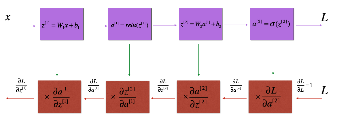
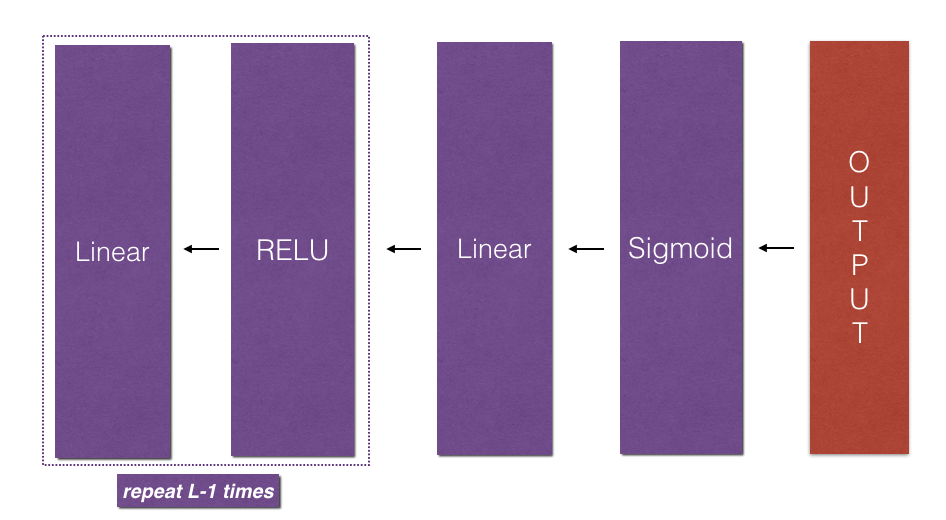
L層模型反向傳播
L層模型反向傳播的流程,如圖所示:
使用這個公式實現反向傳播:
$$grads[“dW” + str(l)] = dW^{[l]}\tag{9} $$
def L_model_backward(AL, Y, caches):
    """
    實現[線性->RELU] * (L-1) ->線性-> SIGMOID組的反向傳播。
    :param AL: 概率向量,正向傳播的輸出(L_model_forward())
    :param Y: true“label”vector(如果非cat,則包含0)
    :param caches: 緩存包含列表:
                所有的緩存來自linear_activation_forward()的"relu" (它是caches[l], for l in range(L-1) i.e l = 0...L-2)
                緩存來自linear_activation_forward()的"sigmoid" (它是caches[L-1])
    :return: 梯度字典:
             grads["dA" + str(l)]
             grads["dW" + str(l)]
             grads["db" + str(l)]
    """
    grads = {}
    L = len(caches)  # the number of layers
    m = AL.shape[1]
    Y = Y.reshape(AL.shape)  # after this line, Y is the same shape as AL

    # Initializing the backpropagation
    dAL = - (np.divide(Y, AL) - np.divide(1 - Y, 1 - AL))

    # Lth layer (SIGMOID -> LINEAR) gradients. Inputs: "AL, Y, caches". Outputs: "grads["dAL"], grads["dWL"], grads["dbL"]
    current_cache = caches[L - 1]
    grads["dA" + str(L - 1)], grads["dW" + str(L)], grads["db" + str(L)] = linear_activation_backward(dAL,
                                                                                                      current_cache,
                                                                                                      activation="sigmoid")

    for l in reversed(range(L - 1)):
        # lth layer: (RELU -> LINEAR) gradients.
        current_cache = caches[l]
        dA_prev_temp, dW_temp, db_temp = linear_activation_backward(grads["dA" + str(l + 1)], current_cache,
                                                                    activation="relu")
        grads["dA" + str(l)] = dA_prev_temp
        grads["dW" + str(l + 1)] = dW_temp
        grads["db" + str(l + 1)] = db_temp

    return grads
更新模型參數
使用梯度下降來更新模型的參數,使用到的公式如下:
$$ W^{[l]} = W^{[l]} - \alpha \text{ } dW^{[l]} \tag{10}$$
$$ b^{[l]} = b^{[l]} - \alpha \text{ } db^{[l]} \tag{11}$$
def update_parameters(parameters, grads, learning_rate):
    """
    使用梯度下降來更新參數。
    :param parameters: 包含參數的python字典。
    :param grads: 包含您的梯度的python字典,l_model_back的輸出。
    :param learning_rate: 學習率
    :return:
    parameters -- 包含更新參數的python字典。
                  parameters["W" + str(l)]
                  parameters["b" + str(l)]
    """
    L = len(parameters) // 2  # number of layers in the neural network

    for l in range(L):
        parameters["W" + str(l + 1)] = parameters["W" + str(l + 1)] - learning_rate * grads["dW" + str(l + 1)]
        parameters["b" + str(l + 1)] = parameters["b" + str(l + 1)] - learning_rate * grads["db" + str(l + 1)]
    return parameters
預測正確率
通過傳入數據和對於的標籤,還有模型參數就可以預測數據並計算準確率了。
def predict(X, y, parameters):
    """
    該函數用於預測l層神經網絡的結果。
    :param X: 您想要標記的示例數據集。
    :param y: 正確的標籤
    :param parameters: 訓練模式的參數。
    :return:
     p -- 對給定數據集X的預測。
    """
    m = X.shape[1]
    n = len(parameters) // 2  # 神經網絡中的層數。
    p = np.zeros((1, m))

    # 正向傳播
    probas, caches = L_model_forward(X, parameters)

    # 將檢驗結果轉換爲0/1預測。
    for i in range(0, probas.shape[1]):
        if probas[0, i] > 0.5:
            p[0, i] = 1
        else:
            p[0, i] = 0

    m = float(m)
    print("Accuracy: " + str(np.sum((p == y) / m)))

    return p
兩層神經網絡模型
構建一個具有以下結構的2層神經網絡:LINEAR - > RELU - > LINEAR - > SIGMOID。
def two_layer_model(X, Y, layers_dims, learning_rate=0.0075, num_iterations=3000, print_cost=False):
    """
    實現了兩層神經網絡:LINEAR>RELU->LINEAR->SIGMOID。
    :param X: 輸入數據,形狀(n_x,示例數量)
    :param Y: 真正的“標籤”向量(包含0如果貓,1如果是非貓),形狀(1,例子數量)
    :param layers_dims: 層的維數(n_x, n_h, n_y)
    :param learning_rate: 梯度下降更新規則的學習速率
    :param num_iterations: 優化循環的迭代次數。
    :param print_cost: 如果設置爲True,則每100次迭代將打印成本。
    :return:
    parameters -- 包含W1、W2、b1和b2的字典
    """
    grads = {}
    costs = []
    m = X.shape[1]  # number of examples
    (n_x, n_h, n_y) = layers_dims

    parameters = initialize_parameters(n_x, n_h, n_y)
    W1 = parameters["W1"]
    b1 = parameters["b1"]
    W2 = parameters["W2"]
    b2 = parameters["b2"]

    # 循環(梯度下降)
    for i in range(0, num_iterations):

        # 正向傳播: LINEAR -> RELU -> LINEAR -> SIGMOID
        A1, cache1 = linear_activation_forward(X, W1, b1, activation="relu")
        A2, cache2 = linear_activation_forward(A1, W2, b2, activation="sigmoid")

        # 計算損失
        cost = compute_cost(A2, Y)

        # 初始化反向傳播
        dA2 = - (np.divide(Y, A2) - np.divide(1 - Y, 1 - A2))

        # 反向傳播
        dA1, dW2, db2 = linear_activation_backward(dA2, cache2, activation="sigmoid")
        dA0, dW1, db1 = linear_activation_backward(dA1, cache1, activation="relu")
        grads['dW1'] = dW1
        grads['db1'] = db1
        grads['dW2'] = dW2
        grads['db2'] = db2

        # 更新參數。
        parameters = update_parameters(parameters, grads, learning_rate)
        W1 = parameters["W1"]
        b1 = parameters["b1"]
        W2 = parameters["W2"]
        b2 = parameters["b2"]

        # 打印每100個培訓實例的成本。
        if print_cost and i % 100 == 0:
            print("Cost after iteration {}: {}".format(i, np.squeeze(cost)))
        if print_cost and i % 100 == 0:
            costs.append(cost)

    # plot the cost
    plt.plot(np.squeeze(costs))
    plt.ylabel('cost')
    plt.xlabel('iterations (per tens)')
    plt.title("Learning rate =" + str(learning_rate))
    plt.show()

    return parameters
L層神經網絡模型
構建一個 該該 具有以下結構的L層狀神經網絡:[LINEAR→RELU] * (L-1) - > LINEAR - > SIGMOID
def L_layer_model(X, Y, layers_dims, learning_rate=0.0075, num_iterations=3000, print_cost=False):
    """
    實現一個l層神經網絡:[LINEAR->RELU]*(L-1)->LINEAR->SIGMOID。
    :param X: 數據,形狀的numpy數組(示例的數量,num_px * num_px * 3)
    :param Y: :真正的“標籤”向量(包含0如果貓,1如果是非貓),形狀(1,例子數量)
    :param layers_dims: 包含輸入大小和每層長度的列表(層數+ 1)。
    :param learning_rate: 梯度下降更新規則的學習速率。
    :param num_iterations: 優化循環的迭代次數。
    :param print_cost: 如果是真的,它將每100步打印成本。
    :return:
    parameters -- 由模型學習的參數。他們可以被用來預測。
    """
    costs = []
    parameters = initialize_parameters_deep(layers_dims)
    # 循環(梯度下降)
    for i in range(0, num_iterations):
        # 正向傳播: [LINEAR -> RELU]*(L-1) -> LINEAR -> SIGMOID.
        AL, caches = L_model_forward(X, parameters)
        # 計算損失
        cost = compute_cost(AL, Y)
        # 反向傳播.
        grads = L_model_backward(AL, Y, caches)
        # 更新參數。
        parameters = update_parameters(parameters, grads, learning_rate)

        # 打印每100個培訓實例的成本。
        if print_cost and i % 100 == 0:
            print ("Cost after iteration %i: %f" % (i, cost))
        if print_cost and i % 100 == 0:
            costs.append(cost)

    # plot the cost
    plt.plot(np.squeeze(costs))
    plt.ylabel('cost')
    plt.xlabel('iterations (per tens)')
    plt.title("Learning rate =" + str(learning_rate))
    plt.show()

    return parameters
預測自己的圖像
這個函數是用來預測自己的圖像的,可以自行修剪圖像的大小,滿足訓練時的大小。
def infer_image(my_image,parameters,num_px):
    my_label_y = [1]  # the true class of your image (1 -> cat, 0 -> non-cat)

    fname = "images/" + my_image
    image = np.array(ndimage.imread(fname, flatten=False))
    my_image = scipy.misc.imresize(image, size=(num_px, num_px)).reshape((num_px * num_px * 3, 1))
    my_image = my_image / 255.
    my_predicted_image = predict(my_image, my_label_y, parameters)

    plt.imshow(image)
    print ("y = " + str(np.squeeze(my_predicted_image)) + ", your L-layer model predicts a \"" + classes[
        int(np.squeeze(my_predicted_image)),].decode("utf-8") + "\" picture.")
模型的使用
這使用兩種模型,一個是兩層的模型,另一個是L層的模型。
兩層模型的使用
使用兩層神經網絡優化參數
if __name__ == "__main__":
    # 獲取數據
    train_x_orig, train_y, test_x_orig, test_y, classes = load_dataset()

    # 重塑培訓和測試範例。
    train_x_flatten = train_x_orig.reshape(train_x_orig.shape[0], -1).T
    test_x_flatten = test_x_orig.reshape(test_x_orig.shape[0], -1).T

    # 將數據標準化,使其具有0到1之間的特徵值
    train_x = train_x_flatten / 255.
    test_x = test_x_flatten / 255.

    layers_dims_two = (12288, 7, 1)  # n_x =  num_px * num_px * 3
    parameters = two_layer_model(train_x, train_y, layers_dims_two, num_iterations=2500, print_cost=True)
    predictions_train = predict(train_x, train_y, parameters)
    predictions_test = predict(test_x, test_y, parameters)
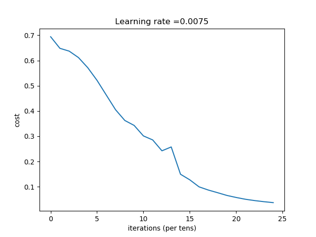
運行後輸出的結果是:
Cost after iteration 0: 0.694163741553
Cost after iteration 100: 0.648266362508
Cost after iteration 200: 0.637126344142
Cost after iteration 300: 0.611710351257
.......
Cost after iteration 2100: 0.0505762788807
Cost after iteration 2200: 0.0453126197353
Cost after iteration 2300: 0.0409255847312
Cost after iteration 2400: 0.0372231796013
Accuracy: 1.0
Accuracy: 0.68
其對應的折線圖:
L層模型的使用
使用深度神經網絡優化參數:
if __name__ == "__main__":
    # 獲取數據
    train_x_orig, train_y, test_x_orig, test_y, classes = load_dataset()

    # 重塑培訓和測試範例。
    train_x_flatten = train_x_orig.reshape(train_x_orig.shape[0], -1).T
    test_x_flatten = test_x_orig.reshape(test_x_orig.shape[0], -1).T

    # 將數據標準化,使其具有0到1之間的特徵值
    train_x = train_x_flatten / 255.
    test_x = test_x_flatten / 255.

    layers_dims_l = [12288, 20, 7, 5, 1]
    parameters = L_layer_model(train_x, train_y, layers_dims_l, num_iterations=2500, print_cost=True)
    pred_train = predict(train_x, train_y, parameters)
    pred_test = predict(test_x, test_y, parameters)
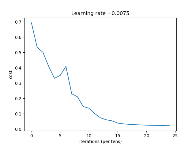
深度神經網絡輸出的日誌如下:
Cost after iteration 0: 0.693828
Cost after iteration 100: 0.533567
Cost after iteration 200: 0.500737
Cost after iteration 300: 0.409495
.....
Cost after iteration 2100: 0.023786
Cost after iteration 2200: 0.022884
Cost after iteration 2300: 0.022056
Cost after iteration 2400: 0.021382
Accuracy: 0.980861244019
Accuracy: 0.7
其對應的折線圖如下:
預測自己的圖像
訓練好的模型也可以用來預測模型自己的圖像:
if __name__ == "__main__":
    # 獲取數據
    train_x_orig, train_y, test_x_orig, test_y, classes = load_dataset()

    # 重塑培訓和測試範例。
    train_x_flatten = train_x_orig.reshape(train_x_orig.shape[0], -1).T
    test_x_flatten = test_x_orig.reshape(test_x_orig.shape[0], -1).T

    # 將數據標準化,使其具有0到1之間的特徵值
    train_x = train_x_flatten / 255.
    test_x = test_x_flatten / 255.

    layers_dims_l = [12288, 20, 7, 5, 1]
    parameters = L_layer_model(train_x, train_y, layers_dims_l, num_iterations=2500, print_cost=True)
    infer_image('images/cat2.jpg', parameters, train_x_orig.shape[1])
預測的結果如下:
y = 1.0, your L-layer model predicts a "cat" picture.
參考資料
- http://deeplearning.ai/
該筆記是學習吳恩達老師的課程寫的。初學者入門,如有理解有誤的,歡迎批評指正!