目錄
@[toc]
常用的激活函數
我們常用的激活函數有sigmoid,tanh,ReLU這三個函數,我們都來學習學習吧。
sigmoid函數
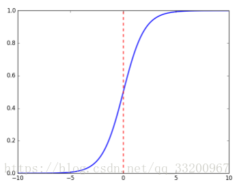
在深度學習中,我們經常會使用到sigmoid函數作爲我們的激活函數,特別是在二分類上,sigmoid函數是比較好的一個選擇,以下就是sigmoid函數的公式:
\(\(sigmoid(x) = \frac{1}{1+e^{-x}}\tag{1}\)\)
sigmoid函數的座標圖是:
sigmoid函數的代碼實現:
import numpy as np

def sigmoid(x):
    s = 1 / (1 + np.exp(-x))
    return s
因爲是使用numpy實現的sigmoid函數的,所以這個sigmoid函數可以計算實數、矢量和矩陣,如下面的就是當x是實數的時候:
if __name__ == '__main__':
    x = 3
    s = sigmoid(x)
    print s
然後會輸出:
0.952574126822
當x是矢量或者矩陣是,計算公式如下:
$$
sigmoid(x) = sigmoid\begin{pmatrix}
x_1 \
x_2 \
… \
x_n \
\end{pmatrix} = \begin{pmatrix}
\frac{1}{1+e^{-x_1}} \
\frac{1}{1+e^{-x_2}} \
… \
\frac{1}{1+e^{-x_n}} \
\end{pmatrix}\tag{2}
$$
使用sigmoid函數如下:
if __name__ == '__main__':
    x = np.array([2, 3, 4])
    s = sigmoid(x)
    print s
輸出的結果是:
[0.88079708 0.95257413 0.98201379]
sigmoid函數的梯度
爲什麼要計算sigmoid函數的梯度,比如當我們在使用反向傳播來計算梯度,以優化損失函數。當使用的激活函數是sigmoid函數就要計算sigmoid函數的梯度了。計算公式如下:
\(\(sigmoid\_derivative(x) = \sigma'(x) = \sigma(x) (1 - \sigma(x))\tag{3}\)\)
Python你代碼實現:
import numpy as np

def sigmoid_derivative(x):
    s = 1 / (1 + np.exp(-x))
    ds = s * (1 - s)
    return ds
當x是實數時,計算如下:
if __name__ == '__main__':
    x = 3
    s = sigmoid_derivative(x)
    print s
輸出結果如下:
0.0451766597309
當x是矩陣或者矢量時,計算如下:
if __name__ == '__main__':
    x = np.array([2, 3, 4])
    s = sigmoid_derivative(x)
    print s
輸出結果如下:
[0.10499359 0.04517666 0.01766271]
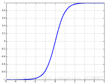
tanh函數
tanh也是一個常用的激活函數,它的公式如下:
\(\(tanh(x) = \frac{e^x-e^{-x}}{e^x+e^{-x}}\tag{4}\)\)
tanh的座標圖是:
tanh的代碼實現:
import numpy as np

def tanh(x):
    s1 = np.exp(x) - np.exp(-x)
    s2 = np.exp(x) + np.exp(-x)
    s = s1 / s2
    return s
爲了方便,這裏把x是實數、矢量或矩陣的情況一起計算了,調用方法如下:
if __name__ == '__main__':
    x = 3
    s = tanh(x)
    print s
    x = np.array([2, 3, 4])
    s = tanh(x)
    print s
以下就是輸出結果:
0.995054753687
[0.96402758 0.99505475 0.9993293 ]
tanh函數的梯度
同樣在這裏我們也要計算tanh函數的梯度,計算公式如下:
$$
tanh_derivative(x) = tanh’(x) = 1 - \tanh^2x = 1- \left(\frac{e^x-e^{-x}}{e^x+e^{-x}}\right)^2\tag{5}
$$
Python代碼實現如下:
import numpy as np

def tanh_derivative(x):
    s1 = np.exp(x) - np.exp(-x)
    s2 = np.exp(x) + np.exp(-x)
    tanh = s1 / s2
    s = 1 - tanh * tanh
    return s
調用方法如下:
if __name__ == '__main__':
    x = 3
    s = tanh_derivative(x)
    print s
    x = np.array([2, 3, 4])
    s = tanh_derivative(x)
    print s
輸出結果如下:
0.00986603716544
[0.07065082 0.00986604 0.00134095]
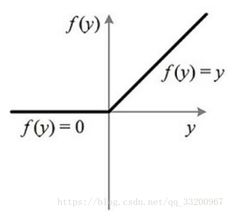
ReLU函數
ReLU是目前深度學習最常用的一個激活函數,數學公式如下:
\(\(relu(x) = max(0,x)=\left\{\begin{matrix}x,& \text{if} \quad x > 0 \\ 0,& \text{if} \quad x \leq0\end{matrix}\right.\tag{6}\)\)
其對應的座標圖爲:
Python代碼的實現:
import numpy as np

def relu(x):
    s = np.where(x < 0, 0, x)
    return s
調用方式如下:
if __name__ == '__main__':
    x = -1
    s = relu(x)
    print s
    x = np.array([2, -3, 1])
    s = relu(x)
    print s
輸出結果如下:
0
[2 0 1]
圖像轉矢量
爲了提高訓練是的計算速度,一般會把圖像轉成矢量,一張三通道的圖像的格式是\((width, height, 3)\)會轉成\((width*height*3, 1)\),我們使用Python代碼嘗試一下:
import numpy as np

def image2vector(image):
    v = image.reshape((image.shape[0] * image.shape[1] * image.shape[2], 1))
    return v
調用方法如下:
if __name__ == '__main__':
    image = np.array([[[0.67826139, 0.29380381],
                       [0.90714982, 0.52835647],
                       [0.4215251, 0.45017551]],

                      [[0.92814219, 0.96677647],
                       [0.85304703, 0.52351845],
                       [0.19981397, 0.27417313]],

                      [[0.60659855, 0.00533165],
                       [0.10820313, 0.49978937],
                       [0.34144279, 0.94630077]]])
    vector = image2vector(image)
    print "image shape is :", image.shape
    print "vector shape is :", vector.shape
    print "vector is :" + str(image2vector(image))
輸出結果如下:
image shape is : (3, 3, 2)
vector shape is : (18, 1)
vector is :[[0.67826139]
 [0.29380381]
 [0.90714982]
 [0.52835647]
 [0.4215251 ]
 [0.45017551]
 [0.92814219]
 [0.96677647]
 [0.85304703]
 [0.52351845]
 [0.19981397]
 [0.27417313]
 [0.60659855]
 [0.00533165]
 [0.10820313]
 [0.49978937]
 [0.34144279]
 [0.94630077]]
規範化行
在深度學習中通過規範化行,可以使模型收斂得更快。它的計算公式如下:
$$
x = \begin{bmatrix}
0 & 3 & 4 \
2 & 6 & 4 \
\end{bmatrix}\tag{7}
$$ then
$$
| x| = np.linalg.norm(x, axis = 1, keepdims = True) = \begin{bmatrix}
5 \
\sqrt{56} \
\end{bmatrix}\tag{8}
$$and
$$ x_normalized = \frac{x}{| x|} = \begin{bmatrix}
0 & \frac{3}{5} & \frac{4}{5} \
\frac{2}{\sqrt{56}} & \frac{6}{\sqrt{56}} & \frac{4}{\sqrt{56}} \
\end{bmatrix}\tag{9}
$$
Python代碼實現:
import numpy as np

def normalizeRows(x):
    x_norm = np.linalg.norm(x, axis=1, keepdims=True)
    print "x_norm = ", x_norm
    x = x / x_norm
    return x
調用該函數:
if __name__ == '__main__':
    x = np.array([
        [0, 3, 4],
        [1, 6, 4]])
    print "normalizeRows(x) = " + str(normalizeRows(x))
輸出結果如下:
x_norm =  [[5.        ]
 [7.28010989]]
normalizeRows(x) = [[0.         0.6        0.8       ]
 [0.13736056 0.82416338 0.54944226]]
廣播和softmax函數
廣播是將較小的矩陣“廣播”到較大矩陣相同的形狀尺度上,使它們對等以可以進行數學計算。注意的是較小的矩陣要是較大矩陣的倍數,否則無法使用廣播。
以下就是softmax函數,這函數在計算的過程就使用到了廣播的性質。softmax函數的公式如下:
$$ x \in \mathbb{R}^{1\times n} \text{, } softmax(x) = softmax(\begin{bmatrix}
x_1 &&
x_2 &&
… &&
x_n
\end{bmatrix}) = \begin{bmatrix}
\frac{e^{x_1}}{\sum_{j}e^{x_j}} &&
\frac{e^{x_2}}{\sum_{j}e^{x_j}} &&
… &&
\frac{e^{x_n}}{\sum_{j}e^{x_j}}
\end{bmatrix} \tag{10}
$$
$$
x \in \mathbb{R}^{m \times n} \text{, }x_{ij} \quad softmax(x) = softmax\begin{bmatrix}
x_{11} & x_{12} & x_{13} & \dots & x_{1n} \
x_{21} & x_{22} & x_{23} & \dots & x_{2n} \
\vdots & \vdots & \vdots & \ddots & \vdots \
x_{m1} & x_{m2} & x_{m3} & \dots & x_{mn}
\end{bmatrix} = \begin{bmatrix}
\frac{e^{x_{11}}}{\sum_{j}e^{x_{1j}}} & \frac{e^{x_{12}}}{\sum_{j}e^{x_{1j}}} & \frac{e^{x_{13}}}{\sum_{j}e^{x_{1j}}} & \dots & \frac{e^{x_{1n}}}{\sum_{j}e^{x_{1j}}} \
\frac{e^{x_{21}}}{\sum_{j}e^{x_{2j}}} & \frac{e^{x_{22}}}{\sum_{j}e^{x_{2j}}} & \frac{e^{x_{23}}}{\sum_{j}e^{x_{2j}}} & \dots & \frac{e^{x_{2n}}}{\sum_{j}e^{x_{2j}}} \
\vdots & \vdots & \vdots & \ddots & \vdots \
\frac{e^{x_{m1}}}{\sum_{j}e^{x_{mj}}} & \frac{e^{x_{m2}}}{\sum_{j}e^{x_{mj}}} & \frac{e^{x_{m3}}}{\sum_{j}e^{x_{mj}}} & \dots & \frac{e^{x_{mn}}}{\sum_{j}e^{x_{mj}}}
\end{bmatrix} = \begin{pmatrix}
softmax\text{(first row of x)} \
softmax\text{(second row of x)} \
… \
softmax\text{(last row of x)} \
\end{pmatrix} \tag{11}
$$
Python代碼的實現:
import numpy as np

def softmax(x):
    x_exp = np.exp(x)
    x_sum = np.sum(x_exp, axis=1, keepdims=True)
    print "x_sum = ", x_sum
    s = x_exp / x_sum
    return s
調用該函數:
if __name__ == '__main__':
    x = np.array([
        [9, 2, 5, 0, 0],
        [7, 5, 0, 0, 0]])
    print "softmax(x) = " + str(softmax(x))
輸出結果如下:
x_sum =  [[8260.88614278]
 [1248.04631753]]
softmax(x) = [[9.80897665e-01 8.94462891e-04 1.79657674e-02 1.21052389e-04 1.21052389e-04]
 [8.78679856e-01 1.18916387e-01 8.01252314e-04 8.01252314e-04 8.01252314e-04]]
numpy矩陣的運算
numpy計算矩陣的有三種:np.dot(),np.outer(),np.multiply()。它們的運算如下:
# coding=utf-8
import numpy as np

if __name__ == '__main__':
    s1 = [[1,2,3],[4,5,6]]
    s2 = [[2,2],[3,3],[4,4]]
    # 跟線性代數計算矩陣一樣,(1*15)*(15*1)=(1*1)
    dot = np.dot(s1, s2)
    print 'dot = ', dot
    # s1第一個元素跟s2的每一個元素相乘作爲第一行,s1第二個元素跟s2每一個元素相乘作爲第二個元素....
    outer = np.outer(s1, s2)
    print 'outer = ', outer
    x1 = [9, 2, 5, 0, 0, 7, 5, 0, 0, 0, 9, 2, 5, 0, 0]
    x2 = [9, 2, 2, 9, 0, 9, 2, 5, 0, 0, 9, 2, 5, 0, 0]
    # x1中的元素和x2中的元素一一對應相乘
    mul = np.multiply(x1, x2)
    print 'mul = ', mul
輸出結果如下:
dot =  [[20 20]
 [47 47]]
outer =  [[ 2  2  3  3  4  4]
 [ 4  4  6  6  8  8]
 [ 6  6  9  9 12 12]
 [ 8  8 12 12 16 16]
 [10 10 15 15 20 20]
 [12 12 18 18 24 24]]
mul =  [81  4 10  0  0 63 10  0  0  0 81  4 25  0  0]
損失函數
損失用於評估模型的性能。損失越大,你的預測\(\hat{y}\)就越不同於真實的值\(y\)。在深度學習中,您可以使用梯度下降等優化算法來訓練模型並最大限度地降低成本。
L1損失函數
L1損失函數的公式如下:
\(\(L_1(\hat{y}, y) = \sum_{i=0}^m|y^{(i)} - \hat{y}^{(i)}| \tag{12}\)\)
Python代碼實現:
import numpy as np

def L1(yhat, y):
    loss = np.sum(abs(y - yhat))
    return loss
調用該函數:
if __name__ == '__main__':
    yhat = np.array([.9, 0.2, 0.1, .4, .9])
    y = np.array([1, 0, 0, 1, 1])
    print("L1 = " + str(L1(yhat, y)))
輸入結果如下:
L1 = 1.1
L2損失函數
L2損失函數的公式如下:
\(\(L_2(\hat{y},y) = \sum_{i=0}^m(y^{(i)} - \hat{y}^{(i)})^2 \tag{13}\)\)
Python代碼實現:
import numpy as np

def L2(yhat, y):
    loss = np.sum(np.multiply((y - yhat), (y - yhat)))
    return loss
調用該函數:
if __name__ == '__main__':
    yhat = np.array([.9, 0.2, 0.1, .4, .9])
    y = np.array([1, 0, 0, 1, 1])
    print("L2 = " + str(L2(yhat, y)))
輸入結果如下:
L2 = 0.43
參考資料
- https://baike.baidu.com/item/tanh
- https://baike.baidu.com/item/Sigmoid%E5%87%BD%E6%95%B0
- http://deeplearning.ai/
該筆記是學習吳恩達老師的課程寫的。初學者入門,如有理解有誤的,歡迎批評指正!