Table of Contents
@[toc]
Common Activation Functions
We commonly use three activation functions: sigmoid, tanh, and ReLU. Let’s learn about each one.
Sigmoid Function
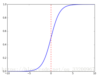
In deep learning, the sigmoid function is often used as an activation function, especially for binary classification. The formula for the sigmoid function is:
\(\(sigmoid(x) = \frac{1}{1+e^{-x}}\tag{1}\)\)
The graph of the sigmoid function is:
Python implementation of sigmoid:
import numpy as np

def sigmoid(x):
    s = 1 / (1 + np.exp(-x))
    return s
This sigmoid function can compute values for real numbers, vectors, and matrices. For real numbers:
if __name__ == '__main__':
    x = 3
    s = sigmoid(x)
    print(s)
Output:
0.952574126822
For vectors or matrices:
$$
sigmoid(x) = sigmoid\begin{pmatrix}
x_1 \
x_2 \
… \
x_n \
\end{pmatrix} = \begin{pmatrix}
\frac{1}{1+e^{-x_1}} \
\frac{1}{1+e^{-x_2}} \
… \
\frac{1}{1+e^{-x_n}} \
\end{pmatrix}\tag{2}
$$
Example usage:
if __name__ == '__main__':
    x = np.array([2, 3, 4])
    s = sigmoid(x)
    print(s)
Output:
[0.88079708 0.95257413 0.98201379]
Sigmoid Gradient
To use backpropagation for optimizing the loss function, we need to compute the gradient of the sigmoid function. The formula is:
\(\(sigmoid\_derivative(x) = \sigma'(x) = \sigma(x) (1 - \sigma(x))\tag{3}\)\)
Python implementation:
import numpy as np

def sigmoid_derivative(x):
    s = 1 / (1 + np.exp(-x))
    ds = s * (1 - s)
    return ds
Example usage:
if __name__ == '__main__':
    x = 3
    s = sigmoid_derivative(x)
    print(s)
Output:
0.0451766597309
For vectors or matrices:
if __name__ == '__main__':
    x = np.array([2, 3, 4])
    s = sigmoid_derivative(x)
    print(s)
Output:
[0.10499359 0.04517666 0.01766271]
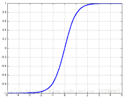
Tanh Function
Tanh is another commonly used activation function. Its formula is:
\(\(tanh(x) = \frac{e^x-e^{-x}}{e^x+e^{-x}}\tag{4}\)\)
The graph of the tanh function is:
Python implementation:
import numpy as np

def tanh(x):
    s1 = np.exp(x) - np.exp(-x)
    s2 = np.exp(x) + np.exp(-x)
    s = s1 / s2
    return s
Example usage for real numbers, vectors, and matrices:
if __name__ == '__main__':
    x = 3
    s = tanh(x)
    print(s)
    x = np.array([2, 3, 4])
    s = tanh(x)
    print(s)
Output:
0.995054753687
[0.96402758 0.99505475 0.9993293 ]
Tanh Gradient
The gradient of the tanh function is calculated as:
$$
tanh_derivative(x) = tanh’(x) = 1 - \tanh^2x = 1- \left(\frac{e^x-e^{-x}}{e^x+e^{-x}}\right)^2\tag{5}
$$
Python implementation:
import numpy as np

def tanh_derivative(x):
    s1 = np.exp(x) - np.exp(-x)
    s2 = np.exp(x) + np.exp(-x)
    tanh = s1 / s2
    s = 1 - tanh * tanh
    return s
Example usage:
if __name__ == '__main__':
    x = 3
    s = tanh_derivative(x)
    print(s)
    x = np.array([2, 3, 4])
    s = tanh_derivative(x)
    print(s)
Output:
0.00986603716544
[0.07065082 0.00986604 0.00134095]
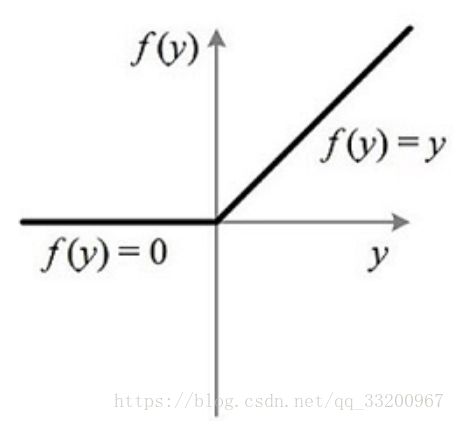
ReLU Function
ReLU is currently the most commonly used activation function in deep learning. Its formula is:
\(\(relu(x) = max(0,x)=\left\{\begin{matrix}x,& \text{if} \quad x > 0 \\ 0,& \text{if} \quad x \leq0\end{matrix}\right.\tag{6}\)\)
The graph of the ReLU function is:
Python implementation:
import numpy as np

def relu(x):
    s = np.where(x < 0, 0, x)
    return s
Example usage:
if __name__ == '__main__':
    x = -1
    s = relu(x)
    print(s)
    x = np.array([2, -3, 1])
    s = relu(x)
    print(s)
Output:
0
[2 0 1]
Image to Vector
To improve training speed, images are often converted to vectors. A 3-channel image with dimensions \((width, height, 3)\) becomes \((width*height*3, 1)\).
Python implementation:
import numpy as np

def image2vector(image):
    v = image.reshape((image.shape[0] * image.shape[1] * image.shape[2], 1))
    return v
Example usage:
if __name__ == '__main__':
    image = np.array([[[0.67826139, 0.29380381],
                       [0.90714982, 0.52835647],
                       [0.4215251, 0.45017551]],

                      [[0.92814219, 0.96677647],
                       [0.85304703, 0.52351845],
                       [0.19981397, 0.27417313]],

                      [[0.60659855, 0.00533165],
                       [0.10820313, 0.49978937],
                       [0.34144279, 0.94630077]]])
    vector = image2vector(image)
    print("image shape is :", image.shape)
    print("vector shape is :", vector.shape)
    print("vector is :" + str(image2vector(image)))
Output:
image shape is : (3, 3, 2)
vector shape is : (18, 1)
vector is :[[0.67826139]
 [0.29380381]
 [0.90714982]
 [0.52835647]
 [0.4215251 ]
 [0.45017551]
 [0.92814219]
 [0.96677647]
 [0.85304703]
 [0.52351845]
 [0.19981397]
 [0.27417313]
 [0.60659855]
 [0.00533165]
 [0.10820313]
 [0.49978937]
 [0.34144279]
 [0.94630077]]
Normalize Rows
Normalizing rows helps models converge faster. The formula for normalization is:
For a matrix \(x\):
$$
x = \begin{bmatrix}
0 & 3 & 4 \
2 & 6 & 4 \
\end{bmatrix}\tag{7}
$$
First, compute the L2 norm (magnitude) of each row:
$$
| x| = np.linalg.norm(x, axis = 1, keepdims = True) = \begin{bmatrix}
5 \
\sqrt{56} \
\end{bmatrix}\tag{8}
$$
Then normalize each row by dividing by its norm:
$$ x_normalized = \frac{x}{| x|} = \begin{bmatrix}
0 & \frac{3}{5} & \frac{4}{5} \
\frac{2}{\sqrt{56}} & \frac{6}{\sqrt{56}} & \frac{4}{\sqrt{56}} \
\end{bmatrix}\tag{9}
$$
Python implementation:
import numpy as np

def normalizeRows(x):
    x_norm = np.linalg.norm(x, axis=1, keepdims=True)
    print("x_norm = ", x_norm)
    x = x / x_norm
    return x
Example usage:
if __name__ == '__main__':
    x = np.array([
        [0, 3, 4],
        [1, 6, 4]])
    print("normalizeRows(x) = " + str(normalizeRows(x)))
Output:
x_norm =  [[5.        ]
 [7.28010989]]
normalizeRows(x) = [[0.         0.6        0.8       ]
 [0.13736056 0.82416338 0.54944226]]
Broadcasting and Softmax Function
Broadcasting scales smaller matrices to match the shape of larger matrices for element-wise operations. The softmax function uses broadcasting.
Softmax for a vector:
$$ x \in \mathbb{R}^{1\times n} \text{, } softmax(x) = softmax(\begin{bmatrix}
x_1 &&
x_2 &&
… &&
x_n
\end{bmatrix}) = \begin{bmatrix}
\frac{e^{x_1}}{\sum_{j}e^{x_j}} &&
\frac{e^{x_2}}{\sum_{j}e^{x_j}} &&
… &&
\frac{e^{x_n}}{\sum_{j}e^{x_j}}
\end{bmatrix} \tag{10}
$$
Softmax for a matrix:
$$
x \in \mathbb{R}^{m \times n} \text{, }x_{ij} \quad softmax(x) = softmax\begin{bmatrix}
x_{11} & x_{12} & x_{13} & \dots & x_{1n} \
x_{21} & x_{22} & x_{23} & \dots & x_{2n} \
\vdots & \vdots & \vdots & \ddots & \vdots \
x_{m1} & x_{m2} & x_{m3} & \dots & x_{mn}
\end{bmatrix} = \begin{bmatrix}
\frac{e^{x_{11}}}{\sum_{j}e^{x_{1j}}} & \frac{e^{x_{12}}}{\sum_{j}e^{x_{1j}}} & \frac{e^{x_{13}}}{\sum_{j}e^{x_{1j}}} & \dots & \frac{e^{x_{1n}}}{\sum_{j}e^{x_{1j}}} \
\frac{e^{x_{21}}}{\sum_{j}e^{x_{2j}}} & \frac{e^{x_{22}}}{\sum_{j}e^{x_{2j}}} & \frac{e^{x_{23}}}{\sum_{j}e^{x_{2j}}} & \dots & \frac{e^{x_{2n}}}{\sum_{j}e^{x_{2j}}} \
\vdots & \vdots & \vdots & \ddots & \vdots \
\frac{e^{x_{m1}}}{\sum_{j}e^{x_{mj}}} & \frac{e^{x_{m2}}}{\sum_{j}e^{x_{mj}}} & \frac{e^{x_{m3}}}{\sum_{j}e^{x_{mj}}} & \dots & \frac{e^{x_{mn}}}{\sum_{j}e^{x_{mj}}}
\end{bmatrix} = \begin{pmatrix}
softmax\text{(first row of x)} \
softmax\text{(second row of x)} \
… \
softmax\text{(last row of x)} \
\end{pmatrix} \tag{11}
$$
Python implementation:
import numpy as np

def softmax(x):
    x_exp = np.exp(x)
    x_sum = np.sum(x_exp, axis=1, keepdims=True)
    print("x_sum = ", x_sum)
    s = x_exp / x_sum
    return s
Example usage:
if __name__ == '__main__':
    x = np.array([
        [9, 2, 5, 0, 0],
        [7, 5, 0, 0, 0]])
    print("softmax(x) = " + str(softmax(x)))
Output:
x_sum =  [[8260.88614278]
 [1248.04631753]]
softmax(x) = [[9.80897665e-01 8.94462891e-04 1.79657674e-02 1.21052389e-04 1.21052389e-04]
 [8.78679856e-01 1.18916387e-01 8.01252314e-04 8.01252314e-04 8.01252314e-04]]
Numpy Matrix Operations
Numpy provides three main matrix operations: np.dot(), np.outer(), and np.multiply().
Dot product (matrix multiplication):
# coding=utf-8
import numpy as np

if __name__ == '__main__':
    s1 = [[1,2,3],[4,5,6]]
    s2 = [[2,2],[3,3],[4,4]]
    dot = np.dot(s1, s2)
    print('dot = ', dot)
Output:
dot =  [[20 20]
 [47 47]]
Outer product (element-wise product of vectors, expanded to matrix):
    outer = np.outer(s1, s2)
    print('outer = ', outer)
Output:
```python
outer = [[ 2 2 3 3 4 4]
[ 4 4 6 6 8 8]
[ 6 6 9 9 12 12]