Table of Contents¶

@[toc]

Introduction to Deep Learning¶

1. AI is likened to the new electricity because, much like electricity did over 100 years ago, AI is transforming multiple industries such as: automotive, agriculture, and supply chains.
2. The recent surge in deep learning can be attributed to: advancements in hardware, particularly GPU computing, which provides greater computational power; its successful application in key domains like advertising, speech recognition, and image recognition; and the digital age, which has generated vast amounts of data.
3. The following diagram illustrates the iterative thinking process across different machine learning approaches:
   
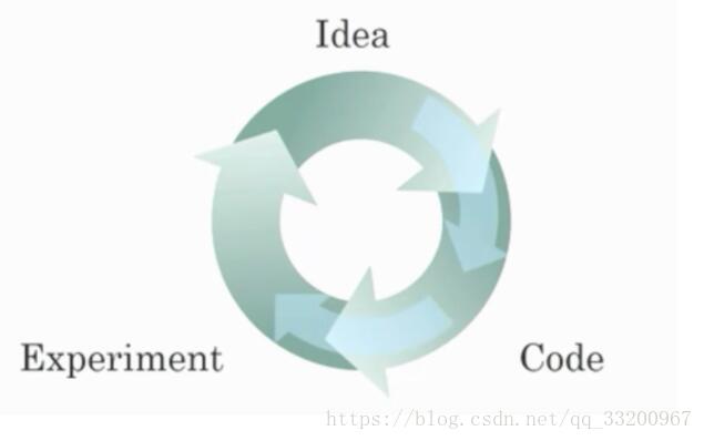
   - This thought map enables rapid idea testing, allowing deep learning engineers to iterate on their concepts more swiftly.
   - It accelerates the team’s ability to refine an idea. New progress in deep learning algorithms allows for better model training even without upgrades to CPU or GPU hardware.
4. Feature engineering is crucial for achieving good performance. While experience helps, building an effective model requires multiple iterations.
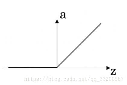
5. The graph of the ReLU activation function is shown below:
   
6. Cat recognition is an example of “unstructured” data. A demographic dataset that counts population, GDP per capita, and economic growth across cities is an example of “structured” data, as opposed to images, audio, or text.
7. RNNs (Recurrent Neural Networks) are used for machine translation because translation is a supervised learning problem that can be trained with sequences. Both the input and output of an RNN are sequences, and translation involves mapping a sequence from one language to another.
8. This hand-drawn graph has the x-axis representing the amount of data and the y-axis representing algorithm performance:
   
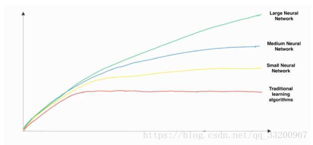
   - The graph shows that increasing training data does not negatively impact algorithm performance; more data is always beneficial for the model.
   - Increasing the size of a neural network typically improves performance. Larger networks generally outperform smaller ones.

Fundamentals of Neural Networks¶

1. A neuron computes a linear function \( z = Wx + b \), followed by an activation function (sigmoid, tanh, ReLU, etc.).
2. When directly computing matrices with numpy, unlike np.dot(a, b), the operations use broadcasting rules. np.dot(a, b) follows standard matrix multiplication.
3. If img is a (32, 32, 3) array representing a 32x32 image with 3 color channels (red, green, blue), reshaping it into a column vector would be: x = img.reshape((32*32*3, 1)).
4. The “Logistic Loss” function is defined as:
   
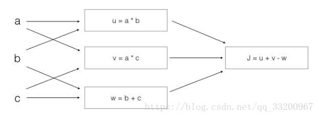
5. The calculation process for the following image is:
   
   [
   \begin{align}
   J &= u + v - w \
   &= (a \cdot b) + (a \cdot c) - (b + c) \
   &= a(b + c) - (b + c) \
   &= (a - 1)(b + c)
   \end{align}
   ]

Shallow Neural Networks¶

1. \( a^{[l(2)]}_{12} \) represents the 12th element of the activation vector in the 2nd layer for a training sample.
2. Each column of matrix \( X \) is a training sample.
3. \( a_4^{[2]} \) denotes the 4th activation output in the 2nd layer.
4. \( a^{[2]} \) represents the activation vector of the 2nd layer.
5. The tanh activation function generally performs better than sigmoid for hidden units because its output ranges between (-1, 1), with a mean closer to zero. This centralizes data for the next layer, simplifying learning.
6. The sigmoid function outputs values between 0 and 1, making it ideal for binary classification (output < 0.5 = class 0, output > 0.5 = class 1). Tanh can also be used, but its values between -1 and 1 are less intuitive for binary tasks.
7. In Logistic Regression (no hidden layers), initializing weights to zero causes the first sample output to be zero. However, the derivative of Logistic Regression depends on the input \( x \) (not zero), so weights will follow \( x \)’s distribution and differ after the second iteration if \( x \) is not a constant vector.
8. When the input to tanh is far from zero, its gradient approaches zero because the slope of tanh is near zero in this region.
9. A single-hidden-layer neural network:
   
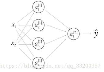
   - \( b^{[1]} \) should have shape (4, 1)
   - \( b^{[2]} \) should have shape (1, 1)
   - \( W^{[1]} \) should have shape (4, 2)
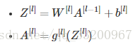
   - \( W^{[2]} \) should have shape (1, 4)
10. For the \( l \)-th layer (where \( 1 \leq l \leq L \)), the correct vectorized forward propagation formula is:
    

Deep Neural Networks¶

1. Using “cache” in forward and backward propagation records values computed during forward passes to enable backward pass calculations via the chain rule.
2. Hyperparameters include: number of iterations, learning rate, number of layers \( L \), and number of hidden units.
3. Deep neural networks can handle more complex input features than shallow networks.
4. The following 4-layer network has 3 hidden layers:
   
   - Layer count: Hidden layers + 1 (input and output layers are not counted as hidden layers).
5. In forward propagation, the activation function (sigmoid, tanh, ReLU, etc.) must be specified because the derivative for backward propagation depends on it.
6. Shallow networks require larger circuits (measured by the number of logic gates) for computations, while deep networks can achieve the same with exponentially smaller circuits.
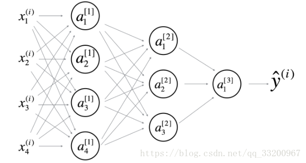
7. A 2-hidden-layer neural network:
   [Image not available in original repository]
   - (i) \( W^{[1]} \) shape: (4, 4) (calculation: \( W^{[l]} = (n^{[l]}, n^{[l-1]}) \)), \( W^{[2]} = (3, 4) \), \( W^{[3]} = (1, 3) \)
   - (ii) \( b^{[1]} \) shape: (4, 1) (calculation: \( b^{[l]} = (n^{[l]}, 1) \)), \( b^{[2]} = (3, 1) \), \( b^{[3]} = (1, 1) \)
8. To initialize model parameters using the layer_dims array [n_x, 4, 3, 2, 1] (4 hidden units in layer 1, etc.):

for i in range(1, len(layer_dims)):
  parameter['W' + str(i)] = np.random.randn(layers[i], layers[i-1]) * 0.01
  parameter['b' + str(i)] = np.random.randn(layers[i], 1) * 0.01

This note is based on studying Andrew Ng’s courses. As a beginner, if there are any misunderstandings, please feel free to correct me!