目錄
@[toc]
前言
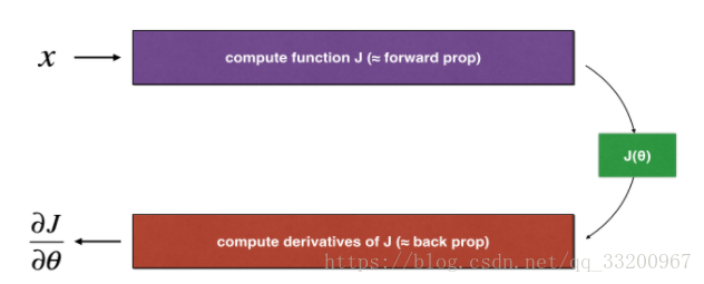
反向傳播計算梯度\(\frac{\partial J}{\partial \theta}\), \(\theta\)表示模型的參數。 \(J\)是使用正向傳播和損失函數來計算的。
計算公式如下:
$$ \frac{\partial J}{\partial \theta} = \lim_{\varepsilon \to 0} \frac{J(\theta + \varepsilon) - J(\theta - \varepsilon)}{2 \varepsilon} \tag{1}$$
因爲向前傳播相對容易實現,所以比較容易獲得正確的結果,確定要計算成本\(J\) 正確。因此,可以通過計算\(J\) 驗證計算\(\frac{\partial J}{\partial \theta}\) 。
一維梯度檢查
一維線性函數\(J(\theta) = \theta x\)。該模型只包含一個實值參數\(\theta\),並採取x作爲輸入。
# coding=utf-8
from testCases import *
from gc_utils import sigmoid, relu, dictionary_to_vector, vector_to_dictionary, gradients_to_vector
def forward_propagation(x, theta):
    """
    實現線性向前傳播(計算J) (J(theta) = theta * x)

    Arguments:
    x -- 一個實值輸入
    theta -- 我們的參數,一個實數。

    Returns:
    J -- 函數J的值, 計算使用公式 J(theta) = theta * x
    """
    J = theta * x
    return J
def backward_propagation(x, theta):
    """
    計算J對的導數

    Arguments:
    x -- 一個實值輸入
    theta -- 我們的參數,一個實數。

    Returns:
    dtheta -- 成本的梯度。
    """

    dtheta = x

    return dtheta
def gradient_check(x, theta, epsilon=1e-7):
    """
    實現反向傳播

    Arguments:
    x -- 一個實值輸入
    theta -- 我們的參數,一個實數
    epsilon -- 用公式對輸入進行微小位移計算近似梯度

    Returns:
    difference -- 近似梯度與反向傳播梯度之間的差異。
    """

    # 用公式的左邊來計算gradapprox(1)
    thetaplus = theta + epsilon  # Step 1
    thetaminus = theta - epsilon  # Step 2
    J_plus = thetaplus * x  # Step 3
    J_minus = thetaminus * x  # Step 4
    gradapprox = (J_plus - J_minus) / (2 * epsilon)  # Step 5

    # :檢查gradapprox是否足夠接近backward_propagation()的輸出
    grad = backward_propagation(x, theta)

    numerator = np.linalg.norm(grad - gradapprox)  # Step 1'
    denominator = np.linalg.norm(grad) + np.linalg.norm(gradapprox)  # Step 2'
    difference = numerator / denominator  # Step 3'

    if difference < 1e-7:
        print ("梯度是正確的!")
    else:
        print ("梯度是錯誤的!")

    return difference
if __name__ == "__main__":
    x, theta = 2, 4
    difference = gradient_check(x, theta)
    print("difference = " + str(difference))
梯度是正確的!
difference = 2.91933588329e-10
## 向前傳播 多維梯度的向前傳播:
def forward_propagation_n(X, Y, parameters):
    """
    實現前面的傳播(並計算成本),如圖3所示。

    Arguments:
    X -- m例的訓練集。
    Y -- m的樣本的標籤
    parameters -- 包含參數的python字典 "W1", "b1", "W2", "b2", "W3", "b3":
                    W1 -- 權重矩陣的形狀(5, 4)
                    b1 -- 偏差的矢量形狀(5, 1)
                    W2 -- 權重矩陣的形狀(3, 5)
                    b2 -- 偏差的矢量形狀(3, 1)
                    W3 -- 權重矩陣的形狀(1, 3)
                    b3 -- 偏差的矢量形狀(1, 1)

    Returns:
    cost -- 成本函數(一個樣本的邏輯成本)
    """

    # 檢索參數
    m = X.shape[1]
    W1 = parameters["W1"]
    b1 = parameters["b1"]
    W2 = parameters["W2"]
    b2 = parameters["b2"]
    W3 = parameters["W3"]
    b3 = parameters["b3"]

    # LINEAR -> RELU -> LINEAR -> RELU -> LINEAR -> SIGMOID
    Z1 = np.dot(W1, X) + b1
    A1 = relu(Z1)
    Z2 = np.dot(W2, A1) + b2
    A2 = relu(Z2)
    Z3 = np.dot(W3, A2) + b3
    A3 = sigmoid(Z3)

    # Cost
    logprobs = np.multiply(-np.log(A3), Y) + np.multiply(-np.log(1 - A3), 1 - Y)
    cost = 1. / m * np.sum(logprobs)

    cache = (Z1, A1, W1, b1, Z2, A2, W2, b2, Z3, A3, W3, b3)

    return cost, cache
def backward_propagation_n(X, Y, cache):
    """
    實現反向傳播。

    Arguments:
    X -- 輸入數據點,形狀(輸入大小,1)
    Y -- true "label"
    cache -- 緩存輸出forward_propagation_n()

    Returns:
    gradients -- 一個字典,它包含了每個參數、激活和預激活變量的成本梯度。
    """

    m = X.shape[1]
    (Z1, A1, W1, b1, Z2, A2, W2, b2, Z3, A3, W3, b3) = cache

    dZ3 = A3 - Y
    dW3 = 1. / m * np.dot(dZ3, A2.T)
    db3 = 1. / m * np.sum(dZ3, axis=1, keepdims=True)

    dA2 = np.dot(W3.T, dZ3)
    dZ2 = np.multiply(dA2, np.int64(A2 > 0))
    dW2 = 1. / m * np.dot(dZ2, A1.T) * 2 # 這有個錯誤
    db2 = 1. / m * np.sum(dZ2, axis=1, keepdims=True)

    dA1 = np.dot(W2.T, dZ2)
    dZ1 = np.multiply(dA1, np.int64(A1 > 0))
    dW1 = 1. / m * np.dot(dZ1, X.T)
    db1 = 4. / m * np.sum(dZ1, axis=1, keepdims=True) # 這有個錯誤

    gradients = {"dZ3": dZ3, "dW3": dW3, "db3": db3,
                 "dA2": dA2, "dZ2": dZ2, "dW2": dW2, "db2": db2,
                 "dA1": dA1, "dZ1": dZ1, "dW1": dW1, "db1": db1}

    return gradients
def gradient_check_n(parameters, gradients, X, Y, epsilon=1e-7):
    """
    檢查backward_propagation_n是否正確地計算了正向傳播的成本輸出的梯度。

    Arguments:
    parameters --包含參數的python字典 "W1", "b1", "W2", "b2", "W3", "b3":
    grad -- backward_propagation_n的輸出包含參數的成本梯度。
    x -- 輸入數據點,形狀(輸入大小,1)
    y -- true "label"
    epsilon -- 用公式對輸入進行微小位移計算近似梯度

    Returns:
    difference -- 近似梯度與反向傳播梯度之間的差異。
    """

    # Set-up variables
    parameters_values, _ = dictionary_to_vector(parameters)
    grad = gradients_to_vector(gradients)
    num_parameters = parameters_values.shape[0]
    J_plus = np.zeros((num_parameters, 1))
    J_minus = np.zeros((num_parameters, 1))
    gradapprox = np.zeros((num_parameters, 1))

    # Compute gradapprox
    for i in range(num_parameters):
        thetaplus = np.copy(parameters_values)  # Step 1
        thetaplus[i][0] = thetaplus[i][0] + epsilon  # Step 2
        J_plus[i], _ = forward_propagation_n(X, Y, vector_to_dictionary(thetaplus))  # Step 3

        thetaminus = np.copy(parameters_values)  # Step 1
        thetaminus[i][0] = thetaminus[i][0] - epsilon  # Step 2
        J_minus[i], _ = forward_propagation_n(X, Y, vector_to_dictionary(thetaminus))  # Step 3

        # Compute gradapprox[i]
        gradapprox[i] = (J_plus[i] - J_minus[i]) / (2 * epsilon)

    # 通過計算與反向傳播梯度比較差異。
    numerator = np.linalg.norm(grad - gradapprox)  # Step 1'
    denominator = np.linalg.norm(grad) + np.linalg.norm(gradapprox)  # Step 2'
    difference = numerator / denominator  # Step 3'

    if difference > 2e-7:
        print (
            "\033[93m" + "反向傳播有一個錯誤! difference = " + str(difference) + "\033[0m")
    else:
        print (
            "\033[92m" + "你的反向傳播效果非常好! difference = " + str(difference) + "\033[0m")

    return difference
if __name__ == "__main__":
    X, Y, parameters = gradient_check_n_test_case()
    cost, cache = forward_propagation_n(X, Y, parameters)
    gradients = backward_propagation_n(X, Y, cache)
    difference = gradient_check_n(parameters, gradients, X, Y)
反向傳播有一個錯誤! difference = 0.285093156781
dW2 = 1. / m * np.dot(dZ2, A1.T) * 2
db1 = 4. / m * np.sum(dZ1, axis=1, keepdims=True)
dW2 = 1. / m * np.dot(dZ2, A1.T)
db1 = 1. / m * np.sum(dZ1, axis=1, keepdims=True)
你的反向傳播效果非常好! difference = 1.18904178766e-07
>該筆記是學習吳恩達老師的課程寫的。初學者入門,如有理解有誤的,歡迎批評指正!