目錄
@[toc]
前言
如果訓練數據集不夠大,由於深度學習模型具有非常大的靈活性和容量,以至於過度擬合可能是一個嚴重的問題,爲了解決這個問題,引入了正則化的這個方法。要在神經網絡中加入正則化,除了在激活層中加入正則函數,應該dropout也是可以起到正則的效果。我們來試試吧。
前提工作
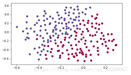
在使用之前,我們還要先導入所需的依賴包,和加載數據,其中有些依賴包可以在這裏下載。
# coding=utf-8
import matplotlib.pyplot as plt
from reg_utils import compute_cost, predict, forward_propagation, backward_propagation, update_parameters
from reg_utils import sigmoid, relu, initialize_parameters, load_2D_dataset
from testCases import *

# 加載數據
train_X, train_Y, test_X, test_Y = load_2D_dataset()
以下就是我們使用到的數據:
模型函數
在這裏編寫一個model函數,來測試和對比以下三種情況:
- 無正則化的情況
- 使用有正則化的激活激活函數
- 使用dropout
def model(X, Y, learning_rate=0.3, num_iterations=30000, print_cost=True, lambd=0, keep_prob=1):
    """
    實現一個三層神經網絡: LINEAR->RELU->LINEAR->RELU->LINEAR->SIGMOID.

    Arguments:
    X -- 輸入數據、形狀(輸入大小、樣本數量)
    Y -- 真正的“標籤”向量(紅點的藍色點/ 0),形狀(輸出大小,樣本數量)
    learning_rate -- 學習速率的優化
    num_iterations -- 優化循環的迭代次數。
    print_cost -- 如果是真的,打印每10000次迭代的成本。
    lambd -- 正則化超參數,標量
    keep_prob - 在dropout過程中保持神經元活躍的概率。

    Returns:
    parameters -- 由模型學習的參數。他們可以被用來預測。
    """

    grads = {}
    costs = []  # to keep track of the cost
    m = X.shape[1]  # number of examples
    layers_dims = [X.shape[0], 20, 3, 1]

    # Initialize parameters dictionary.
    parameters = initialize_parameters(layers_dims)

    # Loop (gradient descent)
    for i in range(0, num_iterations):

        # 正向傳播: LINEAR -> RELU -> LINEAR -> RELU -> LINEAR -> SIGMOID.
        if keep_prob == 1:
            a3, cache = forward_propagation(X, parameters)
        elif keep_prob < 1:
            a3, cache = forward_propagation_with_dropout(X, parameters, keep_prob)

        # Cost function
        if lambd == 0:
            cost = compute_cost(a3, Y)
        else:
            cost = compute_cost_with_regularization(a3, Y, parameters, lambd)

        # Backward propagation.
        assert (lambd == 0 or keep_prob == 1)  # 可以同時使用L2正則化和退出,但是這個任務只會一次探索一個。
        if lambd == 0 and keep_prob == 1:
            grads = backward_propagation(X, Y, cache)
        elif lambd != 0:
            grads = backward_propagation_with_regularization(X, Y, cache, lambd)
        elif keep_prob < 1:
            grads = backward_propagation_with_dropout(X, Y, cache, keep_prob)

        # Update parameters.
        parameters = update_parameters(parameters, grads, learning_rate)

        # 每10000次迭代打印一次損失。
        if print_cost and i % 10000 == 0:
            print("Cost after iteration {}: {}".format(i, cost))
        if print_cost and i % 1000 == 0:
            costs.append(cost)

    # plot the cost
    plt.plot(costs)
    plt.ylabel('cost')
    plt.xlabel('iterations (x1,000)')
    plt.title("Learning rate =" + str(learning_rate))
    plt.show()

    return parameters
無正則化
下面就測試沒有正則化的情況,直接運行項目就可以了。
if __name__ == "__main__":
    parameters = model(train_X, train_Y)
    print ("On the training set:")
    predictions_train = predict(train_X, train_Y, parameters)
    print ("On the test set:")
    predictions_test = predict(test_X, test_Y, parameters)
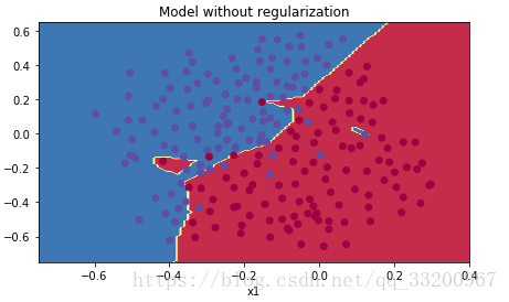
輸出的相關日誌,從中看到訓練的準確率比較高,而測試的準確率比較低,這個是一種過擬合的體現:
Cost after iteration 0: 0.6557412523481002
Cost after iteration 10000: 0.16329987525724216
Cost after iteration 20000: 0.13851642423255986
On the training set:
Accuracy: 0.947867298578
On the test set:
Accuracy: 0.915
以圖表顯示Cost的情況:
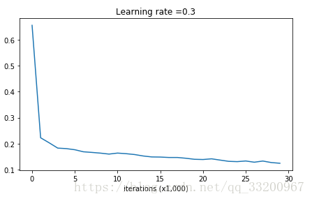
下面是收斂情況,從這個圖像中可以很直觀看出已經存在過擬合情況了:
帶L2正則的激活函數
損失函數
如果L2正則的話,要修改損壞函的計算公式,如下:
損失函數:
\(\(J = -\frac{1}{m} \sum\limits_{i = 1}^{m} \large{(}\small y^{(i)}\log\left(a^{[L](i)}\right) + (1-y^{(i)})\log\left(1- a^{[L](i)}\right) \large{)} \tag{1}\)\)
帶L2正則的損失函數:
\(\(J_{regularized} = \small \underbrace{-\frac{1}{m} \sum\limits_{i = 1}^{m} \large{(}\small y^{(i)}\log\left(a^{[L](i)}\right) + (1-y^{(i)})\log\left(1- a^{[L](i)}\right) \large{)} }_\text{cross-entropy cost} + \underbrace{\frac{1}{m} \frac{\lambda}{2} \sum\limits_l\sum\limits_k\sum\limits_j W_{k,j}^{[l]2} }_\text{L2 regularization cost} \tag{2}\)\)
損失函數的代碼片段如下:
def compute_cost_with_regularization(A3, Y, parameters, lambd):
    """
    用L2正則化實現成本函數。參見上面的公式。

    Arguments:
    A3 -- post-activation,前向傳播輸出,形狀(輸出尺寸,樣本數量)
    Y -- “true”標籤向量,形狀(輸出大小,樣本數量)
    parameters -- 包含模型參數的python字典。

    Returns:
    cost - 正則化損失函數值
    """
    m = Y.shape[1]
    W1 = parameters["W1"]
    W2 = parameters["W2"]
    W3 = parameters["W3"]

    cross_entropy_cost = compute_cost(A3, Y)  # cost的交叉熵。

    L2_regularization_cost = (1 / m) * (lambd / 2) * (
    np.sum(np.square(W1)) + np.sum(np.square(W2)) + np.sum(np.square(W3)))

    cost = cross_entropy_cost + L2_regularization_cost

    return cost
反向傳播
反向傳播所需的更改以考慮正則化。這些變化只涉及dW1,dW2和dW3。對於每一個添加正則化項的梯度(\(\frac{d}{dW} ( \frac{1}{2}\frac{\lambda}{m} W^2) = \frac{\lambda}{m} W\))
def backward_propagation_with_regularization(X, Y, cache, lambd):
    """
    實現基線模型的反向傳播,我們添加了L2正則化。

    Arguments:
    X -- 輸入數據集,形狀(輸入大小,樣本數量)
    Y -- “true”標籤向量,形狀(輸出大小,樣本數量)
    cache -- 緩存輸出forward_propagation()
    lambd -- 正則化超參數,標量

    Returns:
    gradients -- 一個具有對每個參數、激活和預激活變量的梯度的字典。
    """

    m = X.shape[1]
    (Z1, A1, W1, b1, Z2, A2, W2, b2, Z3, A3, W3, b3) = cache

    dZ3 = A3 - Y

    dW3 = 1. / m * np.dot(dZ3, A2.T) + (lambd / m) * W3
    db3 = 1. / m * np.sum(dZ3, axis=1, keepdims=True)

    dA2 = np.dot(W3.T, dZ3)
    dZ2 = np.multiply(dA2, np.int64(A2 > 0))
    dW2 = 1. / m * np.dot(dZ2, A1.T) + (lambd / m) * W2
    db2 = 1. / m * np.sum(dZ2, axis=1, keepdims=True)

    dA1 = np.dot(W2.T, dZ2)
    dZ1 = np.multiply(dA1, np.int64(A1 > 0))
    dW1 = 1. / m * np.dot(dZ1, X.T) + (lambd / m) * W1
    db1 = 1. / m * np.sum(dZ1, axis=1, keepdims=True)

    gradients = {"dZ3": dZ3, "dW3": dW3, "db3": db3, "dA2": dA2,
                 "dZ2": dZ2, "dW2": dW2, "db2": db2, "dA1": dA1,
                 "dZ1": dZ1, "dW1": dW1, "db1": db1}

    return gradients
然後運行帶有L2正則的模型,如下:
if __name__ == "__main__":
    parameters = model(train_X, train_Y, lambd=0.7)
    print ("On the train set:")
    predictions_train = predict(train_X, train_Y, parameters)
    print ("On the test set:")
    predictions_test = predict(test_X, test_Y, parameters)
輸出的日誌信息如下,從日誌信息來看,模型收斂得挺好,沒有過擬合的情況:
Cost after iteration 0: 0.6974484493131264
Cost after iteration 10000: 0.2684918873282239
Cost after iteration 20000: 0.2680916337127301
On the train set:
Accuracy: 0.938388625592
On the test set:
Accuracy: 0.93
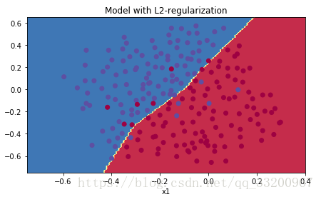
使用圖表來顯示Cost的話,如下:
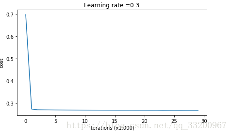
下面是收斂情況,從這個圖像來看,沒有出現過擬合的情況:
L2正則化實際上在做什麼:
L2正則化依賴於這樣的假設,即具有較小權重的模型比具有較大權重的模型更簡單。因此,通過懲罰成本函數中權重的平方值,可以將所有權重驅動到較小的值。擁有大權重的成本太高了!這導致更平滑的模型,其中輸入變化時輸出變化更慢。
L2正則化對以下內容的影響:
- 成本計算:
- 在成本中增加了正則化項。
- 反向傳播功能:
- 在權重矩陣的梯度上有額外的項。
- 權重變小(“權重衰減”):
- 權重被推到較小的值。
Dropout
Dropout是一種廣泛使用的專門針對深度學習的正規化技術。 它在每次迭代中隨機關閉一些神經元。具體流程如下:
def forward_propagation_with_dropout(X, parameters, keep_prob=0.5):
    """
    實現了向前傳播: LINEAR -> RELU + DROPOUT -> LINEAR -> RELU + DROPOUT -> LINEAR -> SIGMOID.

    Arguments:
    X -- 輸入數據集,形狀(2,樣本數量)
    parameters -- 包含參數的python字典 "W1", "b1", "W2", "b2", "W3", "b3":
                    W1 -- 形狀權重矩陣(20,2)
                    b1 -- 形狀偏差向量(20,1)
                    W2 -- 形狀權重矩陣(3,20)
                    b2 -- 形狀的偏差向量(3,1)
                    W3 -- 形狀權重矩陣(1,3)
                    b3 -- 形狀的偏差向量(1,1)
    keep_prob - 在dropout過程中保持神經元活躍的概率。

    Returns:
    A3 -- 最後一個激活值,向前傳播的輸出,形狀(1,1)
    cache -- 元組,用於計算反向傳播的信息。
    """

    np.random.seed(1)

    # retrieve parameters
    W1 = parameters["W1"]
    b1 = parameters["b1"]
    W2 = parameters["W2"]
    b2 = parameters["b2"]
    W3 = parameters["W3"]
    b3 = parameters["b3"]

    # LINEAR -> RELU -> LINEAR -> RELU -> LINEAR -> SIGMOID
    Z1 = np.dot(W1, X) + b1
    A1 = relu(Z1)
    D1 = np.random.rand(A1.shape[0], A1.shape[1])  # Step 1: 初始化矩陣 D1
    D1 = (D1 < keep_prob)  # Step 2: 將D1的條目轉換爲0或1(使用keep_prob作爲閾值)
    A1 = np.multiply(A1, D1)  # Step 3: 關閉A1的一些神經元。
    A1 = A1 / keep_prob  # Step 4: 測量那些沒有被關閉的神經元的價值。
    Z2 = np.dot(W2, A1) + b2
    A2 = relu(Z2)
    D2 = np.random.rand(A2.shape[0], A2.shape[1])  # Step 1: 初始化矩陣D2
    D2 = (D2 < keep_prob)  # Step 2: 將D2的條目轉換爲0或1(使用keep_prob作爲閾值)
    A2 = np.multiply(A2, D2)  # Step 3: 關閉A2的一些神經元。
    A2 = A2 / keep_prob  # Step 4: 測量那些沒有被關閉的神經元的價值。
    Z3 = np.dot(W3, A2) + b3
    A3 = sigmoid(Z3)

    cache = (Z1, D1, A1, W1, b1, Z2, D2, A2, W2, b2, Z3, A3, W3, b3)

    return A3, cache
def backward_propagation_with_dropout(X, Y, cache, keep_prob):
    """
    實現我們的基線模型的反向傳播,我們增加了dropout率。

    Arguments:
    X -- 輸入數據集,形狀(2,樣本數量)
    Y -- “true”標籤向量,形狀(輸出大小,樣本數量)
    cache -- 緩存輸出forward_propagation_with_dropout()
    keep_prob - 在dropout過程中保持神經元活躍的概率。

    Returns:
    gradients --一個具有對每個參數、激活和預激活變量的梯度的字典。
    """

    m = X.shape[1]
    (Z1, D1, A1, W1, b1, Z2, D2, A2, W2, b2, Z3, A3, W3, b3) = cache

    dZ3 = A3 - Y
    dW3 = 1. / m * np.dot(dZ3, A2.T)
    db3 = 1. / m * np.sum(dZ3, axis=1, keepdims=True)
    dA2 = np.dot(W3.T, dZ3)

    dA2 = np.multiply(dA2, D2)  # Step 1: 在向前傳播過程中,應用mask D2關閉相同的神經元。
    dA2 = dA2 / keep_prob  # Step 2: 測量那些沒有被關閉的神經元的值。

    dZ2 = np.multiply(dA2, np.int64(A2 > 0))
    dW2 = 1. / m * np.dot(dZ2, A1.T)
    db2 = 1. / m * np.sum(dZ2, axis=1, keepdims=True)

    dA1 = np.dot(W2.T, dZ2)

    dA1 = np.multiply(dA1, D1)  # Step 1: 使用mask D1關閉與轉發傳播時相同的神經元。
    dA1 = dA1 / keep_prob  # Step 2: 測量那些沒有被關閉的神經元的價值。

    dZ1 = np.multiply(dA1, np.int64(A1 > 0))
    dW1 = 1. / m * np.dot(dZ1, X.T)
    db1 = 1. / m * np.sum(dZ1, axis=1, keepdims=True)

    gradients = {"dZ3": dZ3, "dW3": dW3, "db3": db3, "dA2": dA2,
                 "dZ2": dZ2, "dW2": dW2, "db2": db2, "dA1": dA1,
                 "dZ1": dZ1, "dW1": dW1, "db1": db1}

    return gradients
if __name__ == "__main__":
    parameters = model(train_X, train_Y, keep_prob=0.86, learning_rate=0.3)
    print ("On the train set:")
    predictions_train = predict(train_X, train_Y, parameters)
    print ("On the test set:")
    predictions_test = predict(test_X, test_Y, parameters)
Cost after iteration 0: 0.6543912405149825
Cost after iteration 10000: 0.06101698657490559
Cost after iteration 20000: 0.060582435798513114
On the train set:
Accuracy: 0.928909952607
On the test set:
Accuracy: 0.95
| model | train accuracy | test accuracy | 3-layer NN without regularization | 95% | 91.5% |
| 3-layer NN with L2-regularization | 94% | 93% |
| 3-layer NN with dropout | 93% | 95% |
>該筆記是學習吳恩達老師的課程寫的。初學者入門,如有理解有誤的,歡迎批評指正!