Regularization in Neural Networks¶

Table of Contents¶

@[toc]

Introduction¶

If the training dataset is not large enough, due to the high flexibility and capacity of deep learning models, overfitting can be a severe problem. To address this, regularization methods are introduced. In neural networks, besides adding regularization functions in activation layers, dropout also serves a regularization purpose. Let’s explore this.

Prerequisites¶

Before starting, we need to import the required libraries and load the data. Some dependencies can be downloaded from here.

# coding=utf-8
import matplotlib.pyplot as plt
from reg_utils import compute_cost, predict, forward_propagation, backward_propagation, update_parameters
from reg_utils import sigmoid, relu, initialize_parameters, load_2D_dataset
from testCases import *

# Load dataset
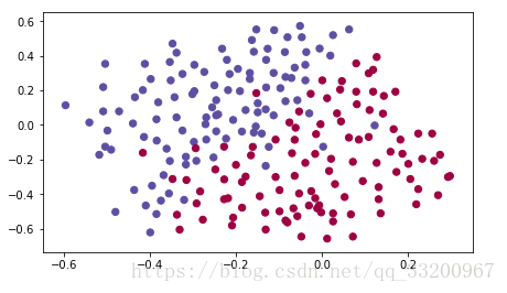
train_X, train_Y, test_X, test_Y = load_2D_dataset()

The dataset used in this example is visualized as follows:

Model Function¶

We’ll implement a model function to test and compare three scenarios:
1. Without regularization
2. With L2-regularized activation function
3. With dropout

def model(X, Y, learning_rate=0.3, num_iterations=30000, print_cost=True, lambd=0, keep_prob=1):
    """
    Implements a three-layer neural network: LINEAR->RELU->LINEAR->RELU->LINEAR->SIGMOID.

    Arguments:
    X -- Input data, shape (input size, number of examples)
    Y -- True "label" vector (red:1, blue:0), shape (output size, number of examples)
    learning_rate -- Learning rate for optimization
    num_iterations -- Number of iterations in optimization loop
    print_cost -- If True, print cost every 10000 iterations
    lambd -- Regularization hyperparameter (scalar)
    keep_prob -- Probability of keeping neurons active during dropout

    Returns:
    parameters -- Parameters learned by the model, used for prediction
    """

    grads = {}
    costs = []  # Track cost
    m = X.shape[1]  # Number of examples
    layers_dims = [X.shape[0], 20, 3, 1]

    # Initialize parameters
    parameters = initialize_parameters(layers_dims)

    # Gradient descent loop
    for i in range(num_iterations):

        # Forward propagation: LINEAR -> RELU -> LINEAR -> RELU -> LINEAR -> SIGMOID
        if keep_prob == 1:
            a3, cache = forward_propagation(X, parameters)
        elif keep_prob < 1:
            a3, cache = forward_propagation_with_dropout(X, parameters, keep_prob)

        # Cost function
        if lambd == 0:
            cost = compute_cost(a3, Y)
        else:
            cost = compute_cost_with_regularization(a3, Y, parameters, lambd)

        # Backward propagation
        assert (lambd == 0 or keep_prob == 1)  # Can use L2 and dropout together, but this task explores one at a time
        if lambd == 0 and keep_prob == 1:
            grads = backward_propagation(X, Y, cache)
        elif lambd != 0:
            grads = backward_propagation_with_regularization(X, Y, cache, lambd)
        elif keep_prob < 1:
            grads = backward_propagation_with_dropout(X, Y, cache, keep_prob)

        # Update parameters
        parameters = update_parameters(parameters, grads, learning_rate)

        # Print cost every 10000 iterations
        if print_cost and i % 10000 == 0:
            print("Cost after iteration {}: {}".format(i, cost))
        if print_cost and i % 1000 == 0:
            costs.append(cost)

    # Plot cost
    plt.plot(costs)
    plt.ylabel('cost')
    plt.xlabel('iterations (x1,000)')
    plt.title("Learning rate = " + str(learning_rate))
    plt.show()

    return parameters

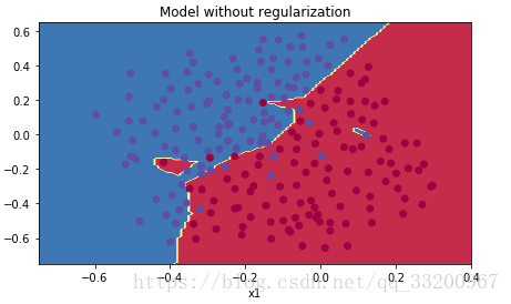
Without Regularization¶

Run the model without regularization to observe overfitting:

if __name__ == "__main__":
    parameters = model(train_X, train_Y)
    print("On the training set:")
    predictions_train = predict(train_X, train_Y, parameters)
    print("On the test set:")
    predictions_test = predict(test_X, test_Y, parameters)

Output:

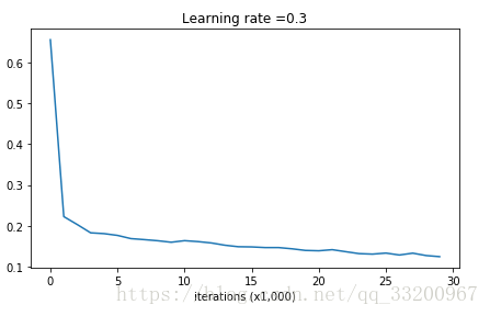
Cost after iteration 0: 0.6557412523481002
Cost after iteration 10000: 0.16329987525724216
Cost after iteration 20000: 0.13851642423255986
On the training set:
Accuracy: 0.947867298578
On the test set:
Accuracy: 0.915

The cost curve shows overfitting:

L2 Regularization on Activation Functions¶

Loss Function¶

For L2 regularization, we modify the loss function:

Standard cross-entropy cost:
\(\(J = -\frac{1}{m} \sum\limits_{i = 1}^{m} \left( y^{(i)}\log\left(a^{[L](i)}\right) + (1-y^{(i)})\log\left(1- a^{[L](i)}\right) \right) \tag{1}\)\)

Regularized cross-entropy cost:
\(\(J_{regularized} = \underbrace{-\frac{1}{m} \sum\limits_{i = 1}^{m} \left( y^{(i)}\log\left(a^{[L](i)}\right) + (1-y^{(i)})\log\left(1- a^{[L](i)}\right) \right)}_{\text{cross-entropy cost}} + \underbrace{\frac{1}{m} \frac{\lambda}{2} \sum\limits_l\sum\limits_k\sum\limits_j W_{k,j}^{[l]2}}_{\text{L2 regularization cost}} \tag{2}\)\)

Implementation Code¶

def compute_cost_with_regularization(A3, Y, parameters, lambd):
    """
    Implements the cost function with L2 regularization.

    Arguments:
    A3 -- Post-activation output of forward propagation, shape (output size, number of examples)
    Y -- True label vector, shape (output size, number of examples)
    parameters -- Python dictionary containing parameters W1, W2, W3

    Returns:
    cost -- Regularized cost value
    """
    m = Y.shape[1]
    W1 = parameters["W1"]
    W2 = parameters["W2"]
    W3 = parameters["W3"]

    cross_entropy_cost = compute_cost(A3, Y)  # Cross-entropy cost

    L2_regularization_cost = (1 / m) * (lambd / 2) * (
        np.sum(np.square(W1)) + np.sum(np.square(W2)) + np.sum(np.square(W3)))

    cost = cross_entropy_cost + L2_regularization_cost

    return cost

Backward Propagation with Regularization¶

def backward_propagation_with_regularization(X, Y, cache, lambd):
    """
    Implements backward propagation with L2 regularization.

    Arguments:
    X -- Input dataset, shape (input size, number of examples)
    Y -- True label vector
    cache -- Output from forward_propagation()
    lambd -- Regularization hyperparameter

    Returns:
    gradients -- Dictionary of gradients
    """
    m = X.shape[1]
    (Z1, A1, W1, b1, Z2, A2, W2, b2, Z3, A3, W3, b3) = cache

    dZ3 = A3 - Y
    dW3 = 1. / m * np.dot(dZ3, A2.T) + (lambd / m) * W3
    db3 = 1. / m * np.sum(dZ3, axis=1, keepdims=True)

    dA2 = np.dot(W3.T, dZ3)
    dZ2 = np.multiply(dA2, np.int64(A2 > 0))
    dW2 = 1. / m * np.dot(dZ2, A1.T) + (lambd / m) * W2
    db2 = 1. / m * np.sum(dZ2, axis=1, keepdims=True)

    dA1 = np.dot(W2.T, dZ2)
    dZ1 = np.multiply(dA1, np.int64(A1 > 0))
    dW1 = 1. / m * np.dot(dZ1, X.T) + (lambd / m) * W1
    db1 = 1. / m * np.sum(dZ1, axis=1, keepdims=True)

    gradients = {"dZ3": dZ3, "dW3": dW3, "db3": db3, "dA2": dA2,
                 "dZ2": dZ2, "dW2": dW2, "db2": db2, "dA1": dA1,
                 "dZ1": dZ1, "dW1": dW1, "db1": db1}

    return gradients

Run L2 Regularized Model¶

if __name__ == "__main__":
    parameters = model(train_X, train_Y, lambd=0.7)
    print("On the train set:")
    predictions_train = predict(train_X, train_Y, parameters)
    print("On the test set:")
    predictions_test = predict(test_X, test_Y, parameters)

Output:

Cost after iteration 0: 0.6974484493131264
Cost after iteration 10000: 0.2684918873282239
Cost after iteration 20000: 0.2680916337127301
On the train set:
Accuracy: 0.938388625592
On the test set:
Accuracy: 0.93

Cost curve:

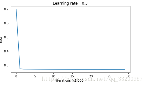
Convergence plot:

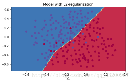
What L2 Regularization Does¶

L2 regularization assumes simpler models have smaller weights. By penalizing weight squares, we drive weights toward smaller values, resulting in smoother models where output changes more slowly with input changes.

Dropout¶

Dropout is a specialized regularization technique for deep learning that randomly deactivates neurons during training.

Dropout Process¶

During forward propagation, some neurons are randomly turned off (masked to 0). During backward propagation, the same neurons are ignored.

Visualization:

Dropout on second hidden layer

Dropout on first and third hidden layers

Forward Propagation with Dropout¶

def forward_propagation_with_dropout(X, parameters, keep_prob=0.5):
    """
    Implements forward propagation with dropout.

    Arguments:
    X -- Input dataset, shape (2, number of examples)
    parameters -- Dictionary containing parameters W1, b1, W2, b2, W3, b3
    keep_prob -- Probability of keeping neurons active

    Returns:
    A3 -- Output of forward propagation
    cache -- Cache for backward propagation
    """
    np.random.seed(1)

    W1 = parameters["W1"]
    b1 = parameters["b1"]
    W2 = parameters["W2"]
    b2 = parameters["b2"]
    W3 = parameters["W3"]
    b3 = parameters["b3"]

    Z1 = np.dot(W1, X) + b1
    A1 = relu(Z1)
    D1 = np.random.rand(A1.shape[0], A1.shape[1])
    D1 = (D1 < keep_prob)
    A1 = np.multiply(A1, D1)
    A1 = A1 / keep_prob  # Scale activation values

    Z2 = np.dot(W2, A1) + b2
    A2 = relu(Z2)
    D2 = np.random.rand(A2.shape[0], A2.shape[1])
    D2 = (D2 < keep_prob)
    A2 = np.multiply(A2, D2)
    A2 = A2 / keep_prob

    Z3 = np.dot(W3, A2) + b3
    A3 = sigmoid(Z3)

    cache = (Z1, D1, A1, W1, b1, Z2, D2, A2, W2, b2, Z3, A3, W3, b3)

    return A3, cache

Backward Propagation with Dropout¶

def backward_propagation_with_dropout(X, Y, cache, keep_prob):
    """
    Implements backward propagation with dropout.

    Arguments:
    X -- Input dataset
    Y -- True label vector
    cache -- Cache from forward_propagation_with_dropout()
    keep_prob -- Probability of keeping neurons active

    Returns:
    gradients -- Dictionary of gradients
    """
    m = X.shape[1]
    (Z1, D1, A1, W1, b1, Z2, D2, A2, W2, b2, Z3, A3, W3, b3) = cache

    dZ3 = A3 - Y
    dW3 = 1. / m * np.dot(dZ3, A2.T)
    db3 = 1. / m * np.sum(dZ3, axis=1, keepdims=True)
    dA2 = np.dot(W3.T, dZ3)

    dA2 = np.multiply(dA2, D2)  # Apply dropout mask
    dA2 = dA2 / keep_prob  # Scale gradients

    dZ2 = np.multiply(dA2, np.int64(A2 > 0))
    dW2 = 1. / m * np.dot(dZ2, A1.T)
    db2 = 1. / m * np.sum(dZ2, axis=1, keepdims=True)

    dA1 = np.dot(W2.T, dZ2)

    dA1 = np.multiply(dA1, D1)  # Apply dropout mask
    dA1 = dA1 / keep_prob  # Scale gradients

    dZ1 = np.multiply(dA1, np.int64(A1 > 0))
    dW1 = 1. / m * np.dot(dZ1, X.T)
    db1 = 1. / m * np.sum(dZ1, axis=1, keepdims=True)

    gradients = {"dZ3": dZ3, "dW3": dW3, "db3": db3, "dA2": dA2,
                 "dZ2": dZ2, "dW2": dW2, "db2": db2, "dA1": dA1,
                 "dZ1": dZ1, "dW1": dW1, "db1": db1}

    return gradients

Run Dropout Model¶

if __name__ == "__main__":
    parameters = model(train_X, train_Y, keep_prob=0.86, learning_rate=0.3)
    print("On the train set:")
    predictions_train = predict(train_X, train_Y, parameters)
    print("On the test set:")
    predictions_test = predict(test_X, test_Y, parameters)

Output:
```text
Cost after iteration 0: 0.6543912405149825
Cost after iteration 10000: 0.0610