Table of Contents
@[toc]
Introduction
A good weight initialization has the following benefits:
- Speeds up the convergence of gradient descent
- Increases the chance that gradient descent converges to a lower training (and generalization) error
Thus, proper initialization is crucial. Here, we test three initialization methods:
- Zero Initialization: Initialize all weight parameters to zero.
- Random Initialization: Use random values to initialize weight parameters.
- He Initialization: A specific initialization formula.
Let’s explore these methods.
Model Function
First, we’ll create a model function to test different weight initialization strategies. We need to import dependencies first. Some packages can be downloaded here.
# coding=utf-8
import numpy as np
from init_utils import compute_loss, forward_propagation, backward_propagation
from init_utils import update_parameters, predict, load_dataset
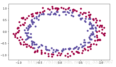
# Load image dataset: blue/red dots in circles
train_X, train_Y, test_X, test_Y = load_dataset()
The dataset looks like this:
Now, let’s implement the model function:
def model(X, Y, learning_rate=0.01, num_iterations=15000, print_cost=True, initialization="he"):
    """
    Implements a three-layer neural network: LINEAR->RELU->LINEAR->RELU->LINEAR->SIGMOID.

    Arguments:
    X -- Input data, shape (2, number of examples)
    Y -- True "label" vector (0 for red dots, 1 for blue dots), shape (1, number of examples)
    learning_rate -- Learning rate of gradient descent
    num_iterations -- Number of iterations to run gradient descent
    print_cost -- If True, print the cost every 1000 iterations
    initialization -- Type of initialization to use ("zeros", "random", or "he")

    Returns:
    parameters -- Parameters learned by the model
    """

    global parameters
    grads = {}
    costs = []  # To track loss
    m = X.shape[1]  # Number of examples
    layers_dims = [X.shape[0], 10, 5, 1]

    # Initialize parameters based on the method
    if initialization == "zeros":
        parameters = initialize_parameters_zeros(layers_dims)
    elif initialization == "random":
        parameters = initialize_parameters_random(layers_dims)
    elif initialization == "he":
        parameters = initialize_parameters_he(layers_dims)

    # Gradient descent loop
    for i in range(0, num_iterations):

        # Forward propagation: LINEAR -> RELU -> LINEAR -> RELU -> LINEAR -> SIGMOID
        a3, cache = forward_propagation(X, parameters)

        # Compute loss
        cost = compute_loss(a3, Y)

        # Backward propagation
        grads = backward_propagation(X, Y, cache)

        # Update parameters
        parameters = update_parameters(parameters, grads, learning_rate)

        # Print cost every 1000 iterations
        if print_cost and i % 1000 == 0:
            print("Cost after iteration {}: {}".format(i, cost))
            costs.append(cost)

    return parameters
Zero Initialization
In neural networks, parameters include:
- Weight matrices \((W^{[1]}, W^{[2]}, ..., W^{[L]})\)
- Bias vectors \((b^{[1]}, b^{[2]}, ..., b^{[L]})\)
def initialize_parameters_zeros(layers_dims):
    """
    Arguments:
    layer_dims -- Python array (list) containing the size of each layer

    Returns:
    parameters -- Python dictionary containing parameters "W1", "b1", ..., "WL", "bL"
                  W1 -- weight matrix of shape (layers_dims[1], layers_dims[0])
                  b1 -- bias vector of shape (layers_dims[1], 1)
                  ...
                  WL -- weight matrix of shape (layers_dims[L], layers_dims[L-1])
                  bL -- bias vector of shape (layers_dims[L], 1)
    """

    parameters = {}
    L = len(layers_dims)  # Number of layers in the network

    for l in range(1, L):
        parameters['W' + str(l)] = np.zeros((layers_dims[l], layers_dims[l - 1]))
        parameters['b' + str(l)] = np.zeros((layers_dims[l], 1))

    return parameters
Testing this will show that the cost doesn’t converge properly because there’s no “symmetry breaking.”
if __name__ == "__main__":
    parameters = model(train_X, train_Y, initialization="zeros")
    print("On the train set:")
    predictions_train = predict(train_X, train_Y, parameters)
    print("On the test set:")
    predictions_test = predict(test_X, test_Y, parameters)
Output Log:
Cost after iteration 0: 0.69314718056
Cost after iteration 1000: 0.69314718056
Cost after iteration 2000: 0.69314718056
... (cost remains constant)
On the train set:
Accuracy: 0.5
On the test set:
Accuracy: 0.5
The cost graph would look like:

Random Initialization
Random initialization breaks symmetry, allowing neurons to learn different features from inputs. We initialize weights randomly but keep biases as zeros.
def initialize_parameters_random(layers_dims):
    """
    Arguments:
    layer_dims -- Python array (list) containing the size of each layer

    Returns:
    parameters -- Python dictionary containing parameters "W1", "b1", ..., "WL", "bL"
                  W1 -- weight matrix of shape (layers_dims[1], layers_dims[0])
                  b1 -- bias vector of shape (layers_dims[1], 1)
                  ...
                  WL -- weight matrix of shape (layers_dims[L], layers_dims[L-1])
                  bL -- bias vector of shape (layers_dims[L], 1)
    """

    parameters = {}
    L = len(layers_dims)  # Number of layers

    for l in range(1, L):
        parameters['W' + str(l)] = np.random.randn(layers_dims[l], layers_dims[l - 1]) * 10
        parameters['b' + str(l)] = np.zeros((layers_dims[l], 1))

    return parameters
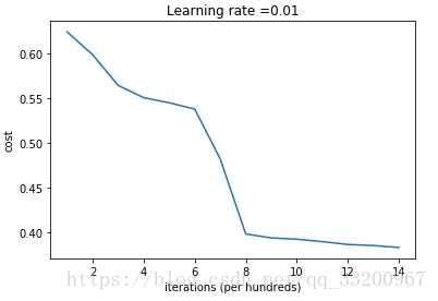
Running this breaks symmetry, and the model starts converging.
if __name__ == "__main__":
    parameters = model(train_X, train_Y, initialization="random")
    print("On the train set:")
    predictions_train = predict(train_X, train_Y, parameters)
    print("On the test set:")
    predictions_test = predict(test_X, test_Y, parameters)
Output Log:
Cost after iteration 0: inf
Cost after iteration 1000: 0.386009576858
Cost after iteration 2000: 0.276065073598
... (cost decreases)
On the train set:
Accuracy: 0.883333333333
On the test set:
Accuracy: 0.85
The cost graph would look like:
He Initialization
He initialization is similar to random initialization but scales weights differently. For ReLU activations, we use \(\sqrt{\frac{2}{\text{dimension of the previous layer}}}\).
def initialize_parameters_he(layers_dims):
    """
    Arguments:
    layer_dims -- Python array (list) containing the size of each layer

    Returns:
    parameters -- Python dictionary containing parameters "W1", "b1", ..., "WL", "bL"
                  W1 -- weight matrix of shape (layers_dims[1], layers_dims[0])
                  b1 -- bias vector of shape (layers_dims[1], 1)
                  ...
                  WL -- weight matrix of shape (layers_dims[L], layers_dims[L-1])
                  bL -- bias vector of shape (layers_dims[L], 1)
    """

    np.random.seed(3)
    parameters = {}
    L = len(layers_dims) - 1  # Number of layers

    for l in range(1, L + 1):
        parameters['W' + str(l)] = np.random.randn(layers_dims[l], layers_dims[l - 1]) * np.sqrt(
            2. / layers_dims[l - 1])
        parameters['b' + str(l)] = np.zeros((layers_dims[l], 1))

    return parameters
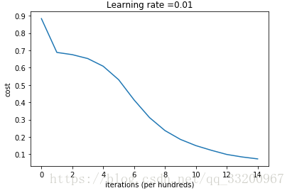
Testing this initialization method:
if __name__ == "__main__":
    parameters = model(train_X, train_Y, initialization="he")
    print("On the train set:")
    predictions_train = predict(train_X, train_Y, parameters)
    print("On the test set:")
    predictions_test = predict(test_X, test_Y, parameters)
Output Log:
Cost after iteration 0: 0.883053746342
Cost after iteration 1000: 0.687982591973
... (cost decreases significantly)
On the train set:
Accuracy: 0.993333333333
On the test set:
Accuracy: 0.96
The cost graph would look like:
Summary
We compare the three initialization methods in the table below:
| Model | Train Accuracy | Problem/Comment |
|---|---|---|
| 3-layer NN with zero init | 50% | Fails to break symmetry |
| 3-layer NN with large random init | 83% | Too large weights |
| 3-layer NN with He init | 99% | Recommended method |
References
- http://deeplearning.ai/
This note is based on Andrew Ng’s course. As a beginner, if there are any misunderstandings, please feel free to comment and correct!