Table of Contents¶

@[toc]

Practical Aspects of Deep Learning¶

1. For 10,000,000 examples, the dataset split is generally 98% training, 1% validation, 1% test.
2. Validation and test datasets usually come from the same distribution.
3. When there are large gaps between the performance of different neural network models, the general solution is to increase the dataset size and add regularization.
4. When the training set error is small but the validation set error is large, increasing the regularization lambda value and expanding the dataset are typically recommended.
5. Increasing the regularization hyperparameter lambda pushes weights towards smaller values, closer to zero.
6. Increasing the parameter keep_prob from (e.g.) 0.5 to 0.6 may reduce regularization effect, potentially leading to lower training set errors.
7. Increasing training data, adding Dropout, and applying regularization techniques can reduce variance (alleviate overfitting).
8. Weight decay is a regularization technique (e.g., L2 regularization) that causes gradient descent to shrink weights in each iteration.
9. We normalize the input data X because it helps the loss function converge faster during optimization.
10. When using the reverse dropout method during testing, dropout (randomly eliminating units) should not be applied, nor should the 1/keep_prob scaling factor used during training calculations.

Optimization Algorithms¶

1. When the input is the 7th example of the 8th minibatch, the activation of the 3rd layer is represented as: \(a^{[3]\{8\}(7)}\).
2. One iteration of Mini-batch Gradient Descent (computed on a single minibatch) is faster than one iteration of Batch Gradient Descent.
3. The optimal minibatch size is usually between 1 and m, not 1 or m. 1) Using a minibatch size of 1 loses vectorization benefits within the minibatch. 2) Using a minibatch size of m results in Batch Gradient Descent, which requires processing the entire training set before completing one iteration.
4. Suppose the cost function J of a learning algorithm is plotted against the number of iterations, as shown:
   
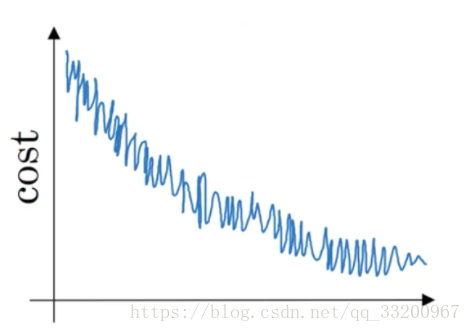
   From the plot, if using Mini-batch Gradient Descent, it appears acceptable. If using Batch Gradient Descent, something is wrong.
5. Suppose the temperature in Casablanca was the same for the first three days of January:
   - January 1st: \(\theta_1 = 10^\circ C\)
   - January 2nd: \(\theta_2 = 10^\circ C\)
   Using exponential weighted averages with \(\beta=0.5\) to track temperature: \(v_0 = 0, v_t = \beta v_{t-1} + (1-\beta)\theta_t\). After 2 days: \(v_2 = 7.5\), and the corrected bias value is: \(v_2^{corrected} = 10\).
6. \(\alpha = e^t \alpha_0\) is not a good learning rate decay method, where t is the epoch number. Better methods include: \(\alpha = 0.95^t \alpha_0\), \(\alpha = \frac{1}{\sqrt{t}} \alpha_0\), or \(\alpha = \frac{1}{1+2t} \alpha_0\).
7. Using exponential weighted averages on London temperature dataset: \(v_{t} = \beta v_{t-1} + (1-\beta)\theta_t\). The red line uses \(\beta=0.9\).
   
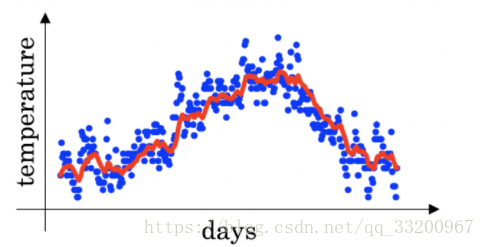
   Increasing \(\beta\) shifts the red line slightly to the right; decreasing \(\beta\) introduces more oscillations around the line.
8. The plot:
   
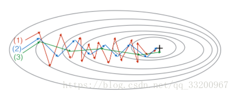
   Shows Gradient Descent, Momentum Gradient Descent (\(\beta=0.5\)), and Momentum Gradient Descent (\(\beta=0.9\)). (1) is Gradient Descent, (2) is Momentum (small \(\beta\)), (3) is Momentum (large \(\beta\)).
9. If Batch Gradient Descent in a deep network takes too long to find parameters minimizing \(\mathcal{J}(W^{[1]},b^{[1]},..., W^{[L]},b^{[L]})\), try: 1) Adjust learning rate \(\alpha\); 2) Better random weight initialization; 3) Use Mini-batch Gradient Descent; 4) Use Adam.
10. Correct statements about Adam: 1) Learning rate \(\alpha\) often needs adjustment; 2) Default hyperparameters are \(\beta_1=0.9, \beta_2=0.999, \varepsilon=10^{-8}\); 3) Adam combines RMSProp and Momentum advantages.

Hyperparameter Tuning, Batch Normalization, and Programming Frameworks¶

1. For searching large hyperparameter spaces, random sampling is preferred over grid search.
2. Not all hyperparameters impact training equally; learning rate is often more critical than others.
3. During hyperparameter search, whether to use “panda” (single model optimization) or “caviar” (parallel model training) depends on available computational resources.
4. For sampling \(\beta\) (momentum hyperparameter) between 0.9 and 0.99:

r = np.random.rand()
beta = 1 - 10**(-r - 1)

5. After finding good hyperparameters, they need re-tuning when network architecture or other hyperparameters change.
6. In Batch Normalization, when applied to the first layer of your neural network, \(z^{[l]}\) is normalized using the formula.
7. In the normalization formula \(z_{norm}^{(i)} = \frac{z^{(i)} - \mu}{\sqrt{\sigma^2 + \varepsilon}}\), \(\varepsilon\) is used to prevent division by zero in \(z^{(i)} - \mu\).
8. For \(\gamma\) and \(\beta\) in Batch Normalization, they can be learned using Adam, Momentum, or RMSprop (not just Gradient Descent) and model the linear transformation of the normalized \(z^{[l]}\).
9. During Batch Normalization, use exponentially weighted averages of \(\mu\) and \(\sigma^2\) over training minibatches for estimation.
10. In deep learning frameworks, even open-source projects benefit from good governance to ensure long-term openness. Programming frameworks allow writing deep learning algorithms with fewer lines of code than low-level languages like Python.