
构建深度神经网络实现猫的二分类

前言
这次使用一个猫的数据集,我们使用深度神经网络来识别这个是猫或者不是猫。
导包
这里导入了两个工具类,可以从这里下载,这里包含了这个函数和用到的数据集,其中用到了h5py,如果读者没有安装的话,要先用pip安装这个库,还有以下用到的库也要安装。
# coding=utf-8
from dnn_utils_v2 import sigmoid, sigmoid_backward, relu, relu_backward
from lr_utils import load_dataset
import numpy as np
import matplotlib.pyplot as plt
import scipy
from scipy import ndimage
初始化网络参数
在网络定义之前,需要先对网络的参数进行初始化,这里分两个来初始化,一个是两层网络的,另一个是L层网络的。
两层网络的初始化
对两层网络的参数初始化要用到输入层的大小、隐藏层的大小、输出层的大小。
def initialize_parameters(n_x, n_h, n_y):
    """
    初始化参数
    :param n_x: 输入层的大小。
    :param n_h: 隐藏层的大小。
    :param n_y: 输出层的大小。
    :return:
     parameters -- 包含您的参数的python字典:
                    W1 -- 形状重量矩阵(n_h, n_x)
                    b1 -- 形状的偏置向量(n_h, 1)
                    W2 -- 形状重量矩阵(n_y, n_h)
                    b2 -- 形状的偏置向量(n_y, 1)
    """
    W1 = np.random.randn(n_h, n_x) * 0.01
    b1 = np.zeros((n_h, 1))
    W2 = np.random.randn(n_y, n_h) * 0.01
    b2 = np.zeros((n_y, 1))

    assert (W1.shape == (n_h, n_x))
    assert (b1.shape == (n_h, 1))
    assert (W2.shape == (n_y, n_h))
    assert (b2.shape == (n_y, 1))

    parameters = {"W1": W1,
                  "b1": b1,
                  "W2": W2,
                  "b2": b2}

    return parameters
L层网络的初始化
对于更深的网络,需要的参数是网络中每一层的尺寸的python数组。相关的计算如下:
| Shape of W | Shape of b | Activation | Shape of Activation | |
|---|---|---|---|---|
| Layer 1 | $(n^{[1]},12288)$ | $(n^{[1]},1)$ | $Z^{[1]} = W^{[1]} X + b^{[1]} $ | $(n^{[1]},209)$ |
| Layer 2 | $(n^{[2]}, n^{[1]})$ | $(n^{[2]},1)$ | $Z^{[2]} = W^{[2]} A^{[1]} + b^{[2]}$ | $(n^{[2]}, 209)$ |
| $\vdots$ | $\vdots$ | $\vdots$ | $\vdots$ | $\vdots$ |
| Layer L-1 | $(n^{[L-1]}, n^{[L-2]})$ | $(n^{[L-1]}, 1)$ | $Z^{[L-1]} = W^{[L-1]} A^{[L-2]} + b^{[L-1]}$ | $(n^{[L-1]}, 209)$ |
| Layer L | $(n^{[L]}, n^{[L-1]})$ | $(n^{[L]}, 1)$ | $Z^{[L]} = W^{[L]} A^{[L-1]} + b^{[L]}$ | $(n^{[L]}, 209)$ |
def initialize_parameters_deep(layer_dims):
    """
    初始化深度参数
    :param layer_dims: 包含我们网络中每一层的尺寸的python数组(列表)。
    :return:
     parameters -- python字典包含参数的"W1", "b1", ..., "WL", "bL":
                    Wl -- 形状权重矩阵(layer_dims[l], layer_dims[l-1])
                    bl -- 形状偏差向量(layer_dims[l], 1)
    """
    parameters = {}
    L = len(layer_dims)  # number of layers in the network

    for l in range(1, L):
        parameters['W' + str(l)] = np.random.randn(layer_dims[l], layer_dims[l - 1]) / np.sqrt(
            layer_dims[l - 1])  # *0.01
        parameters['b' + str(l)] = np.zeros((layer_dims[l], 1))

        assert (parameters['W' + str(l)].shape == (layer_dims[l], layer_dims[l - 1]))
        assert (parameters['b' + str(l)].shape == (layer_dims[l], 1))

    return parameters
正向传播模块
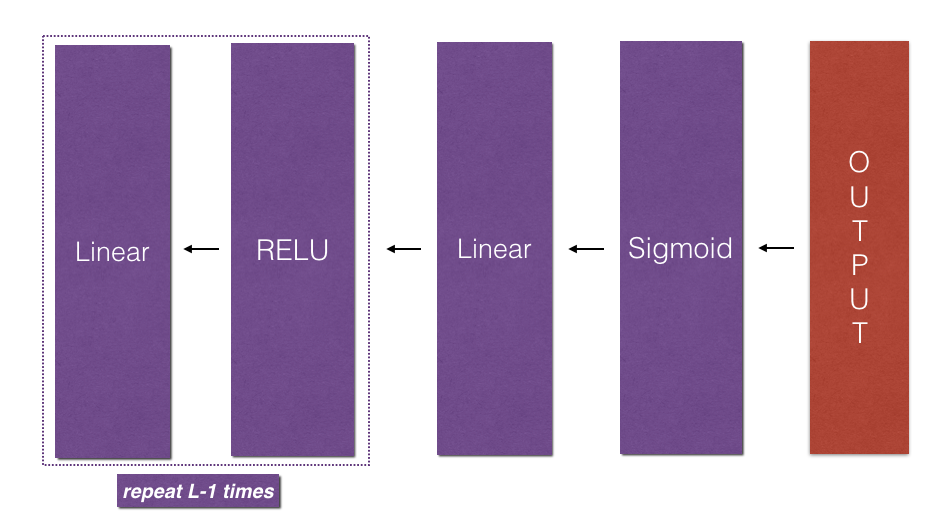
一个完整的神经网络流程是如图所示:
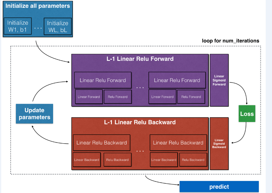
在这一部分,我们要完成的是紫色部分的正向传播,其中包括线性正向传播、线性激活正向传播和完成整个正向传播的L层模型正向传播。
线性正向传播
构建前向传播的线性部分,使用的线性公式如下:
$$
Z^{[l]} = W^{[l]}A^{[l-1]} +b^{[l]}\tag{1}
$$
def linear_forward(A, W, b):
    """
    实现一个层的正向传播的线性部分。
    :param A: 前一层(或输入数据)的激活:(前一层的大小,示例的数量)
    :param W: 权重矩阵:形状的numpy数组(当前层的大小,上一层的大小)
    :param b: 偏置向量,形状的numpy数组(当前层的大小,1)
    :return:
    Z -- 激活函数的输入,也称为预激活参数。
    cache -- :包含“a”、“W”和“b”的python字典;存储用于有效地计算向后传递。
    """
    Z = np.dot(W, A) + b

    assert (Z.shape == (W.shape[0], A.shape[1]))
    cache = (A, W, b)

    return Z, cache
线性激活正向传播
这里使用到了两个激活函数:
- Sigmoid:$\sigma(Z) = \sigma(W A + b) = \frac{1}{ 1 + e^{-(W A + b)}}$
- ReLU:$A = ReLU(Z) = max(0, Z)$
从线性到激活使用到的公式如下:
$$
A^{[l]} = g(Z^{[l]}) = g(W^{[l]}A^{[l-1]} +b^{[l]})\tag{2}
$$
def linear_activation_forward(A_prev, W, b, activation):
    """
    实现线性->激活层的正向传播。
    :param A_prev: 前一层(或输入数据)的激活:(前一层的大小,示例的数量)
    :param W: 权重矩阵:形状的numpy数组(当前层的大小,上一层的大小)
    :param b: 偏置向量,形状的numpy数组(当前层的大小,1)
    :param activation: 在此层中使用的激活,存储为文本字符串:“sigmoid”或“relu”
    :return:
     A -- 激活函数的输出,也称为激活后值。
    cache --包含“线性缓存”和“activation_cache”的python字典;
             存储用于有效地计算向后传递
    """
    if activation == "sigmoid":
        Z, linear_cache = linear_forward(A_prev, W, b)
        A, activation_cache = sigmoid(Z)

    elif activation == "relu":
        Z, linear_cache = linear_forward(A_prev, W, b)
        A, activation_cache = relu(Z)

    assert (A.shape == (W.shape[0], A_prev.shape[1]))
    cache = (linear_cache, activation_cache)

    return A, cache
L层模型正向传播
根据线性正向传播和线性激活正向传播的循环L次,得到一个L层的模型,如下图:
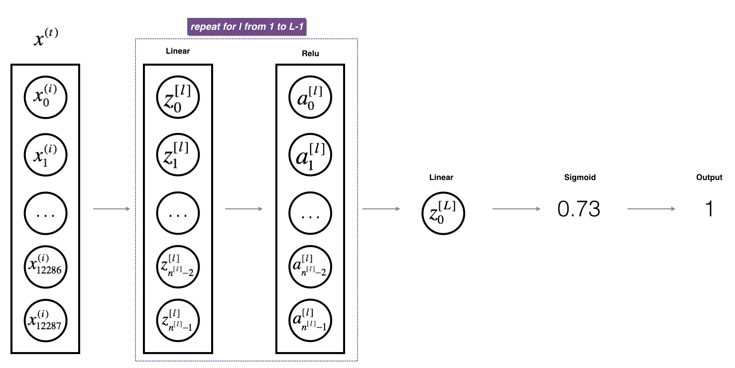
代码中使用到的AL是指公式的$A^{[L]}$:
$$
A^{[L]} = \sigma(Z^{[L]}) = \sigma(W^{[L]} A^{[L-1]} + b^{[L]})\tag{3}
$$
def L_model_forward(X, parameters):
    """
    为[LINEAR->RELU]*(L-1)->LINEAR->SIGMOID计算实现正向传播。
    :param X: 数据,形状的numpy数组(输入大小,示例数量)
    :param parameters: initialize_parameters_deep()的输出
    :return:
    AL -- 最后激活后值
    caches -- 缓存包含列表:
                线性_activation_forward()的每个缓存(其中有L-1,从0到L-1的索引)
    """
    caches = []
    A = X
    L = len(parameters) // 2  # number of layers in the neural network

    # Implement [LINEAR -> RELU]*(L-1). Add "cache" to the "caches" list.
    for l in range(1, L):
        A_prev = A
        A, cache = linear_activation_forward(A_prev, parameters['W' + str(l)], parameters['b' + str(l)],
                                             activation="relu")
        caches.append(cache)

    # Implement LINEAR -> SIGMOID. Add "cache" to the "caches" list.
    AL, cache = linear_activation_forward(A, parameters['W' + str(L)], parameters['b' + str(L)], activation="sigmoid")
    caches.append(cache)

    assert (AL.shape == (1, X.shape[1]))

    return AL, caches
计算损失函数
计算成本函数的公式如下:
$$
cost = -\frac{1}{m} \sum\limits_{i = 1}^{m} (y^{(i)}\log\left(a^{[L] (i)}\right) + (1-y^{(i)})\log\left(1- a^{L}\right)) \tag{4}
$$
def compute_cost(AL, Y):
    """
    实现由公式(7)定义的成本函数。
    :param AL: 对应于你的标签预测的概率向量,形状(1,例子数)
    :param Y: 正确的“标签”矢量(例如:如果非cat,则包含0)、形状(1、示例数量)
    :return:
    cost -- 交叉熵损失
    """
    m = Y.shape[1]

    cost = -(np.sum(np.dot(Y, np.log(AL).T) + np.dot((1 - Y), np.log(1 - AL).T))) / m

    cost = np.squeeze(cost)
    assert (cost.shape == ())

    return cost
反向传播模块
就像向前传播一样,实现反向传播的辅助函数。反向传播用于计算损失函数与参数的梯度
线性反向传播
在反向传播的时候使用到公式如下:
$$
dW^{[l]} = \frac{\partial \mathcal{L} }{\partial W^{[l]}} = \frac{1}{m} dZ^{[l]} A^{[l-1] T} \tag{5}
$$
$$
db^{[l]} = \frac{\partial \mathcal{L} }{\partial b^{[l]}} = \frac{1}{m} \sum_{i = 1}^{m} dZ^{l}\tag{6}
$$
$$
dA^{[l-1]} = \frac{\partial \mathcal{L} }{\partial A^{[l-1]}} = W^{[l] T} dZ^{[l]} \tag{7}
$$
def linear_backward(dZ, cache):
    """
    实现单层(l层)反向传播的线性部分
    :param dZ: 线性输出(当前层l)的成本梯度
    :param cache: 来自当前层的正向传播元组(A_prev, W, b)的值
    :return:
    dA_prev -- 关于激活(前一层l-1)的成本梯度,与A_prev相同。
    dW -- 关于W(当前层l)的成本梯度,与W相同。
    db -- :b(当前层l)的成本梯度,与b相同。
    """
    A_prev, W, b = cache
    m = A_prev.shape[1]

    dW = np.dot(dZ, A_prev.T) / m
    db = np.sum(dZ, axis=1, keepdims=True) / m
    dA_prev = np.dot(W.T, dZ)

    assert (dA_prev.shape == A_prev.shape)
    assert (dW.shape == W.shape)
    assert (db.shape == b.shape)

    return dA_prev, dW, db
线性激活反向传播
在这里使用到的计算公式如下:
$$
dZ^{[l]} = dA^{[l]} * g'(Z^{[l]}) \tag{8}
$$
def linear_activation_backward(dA, cache, activation):
    """
    实现 线性->激活层 的反向传播。
    :param dA: 当前层的激活梯度
    :param cache: 我们存储的值的元组(线性缓存,activation_cache)可以有效地计算反向传播。
    :param activation: 在此层中使用的激活,存储为文本字符串:“sigmoid”或“relu”
    :return:
     dA_prev -- 关于激活(前一层l-1)的成本梯度,与A_prev相同。
    dW -- 关于W(当前层l)的成本梯度,与W相同。
    db -- b(当前层l)的成本梯度,与b相同。
    """
    linear_cache, activation_cache = cache

    if activation == "relu":
        dZ = relu_backward(dA, activation_cache)
        dA_prev, dW, db = linear_backward(dZ, linear_cache)
    elif activation == "sigmoid":
        dZ = sigmoid_backward(dA, activation_cache)
        dA_prev, dW, db = linear_backward(dZ, linear_cache)

    return dA_prev, dW, db
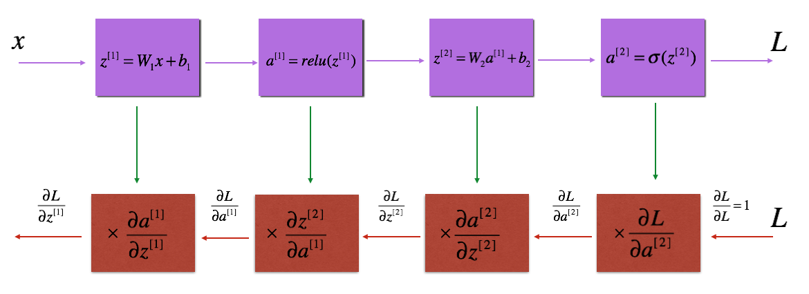
L层模型反向传播
L层模型反向传播的流程,如图所示:
使用这个公式实现反向传播:
$$
grads["dW" + str(l)] = dW^{[l]}\tag{9}
$$
def L_model_backward(AL, Y, caches):
    """
    实现[线性->RELU] * (L-1) ->线性-> SIGMOID组的反向传播。
    :param AL: 概率向量,正向传播的输出(L_model_forward())
    :param Y: true“label”vector(如果非cat,则包含0)
    :param caches: 缓存包含列表:
                所有的缓存来自linear_activation_forward()的"relu" (它是caches[l], for l in range(L-1) i.e l = 0...L-2)
                缓存来自linear_activation_forward()的"sigmoid" (它是caches[L-1])
    :return: 梯度字典:
             grads["dA" + str(l)]
             grads["dW" + str(l)]
             grads["db" + str(l)]
    """
    grads = {}
    L = len(caches)  # the number of layers
    m = AL.shape[1]
    Y = Y.reshape(AL.shape)  # after this line, Y is the same shape as AL

    # Initializing the backpropagation
    dAL = - (np.divide(Y, AL) - np.divide(1 - Y, 1 - AL))

    # Lth layer (SIGMOID -> LINEAR) gradients. Inputs: "AL, Y, caches". Outputs: "grads["dAL"], grads["dWL"], grads["dbL"]
    current_cache = caches[L - 1]
    grads["dA" + str(L - 1)], grads["dW" + str(L)], grads["db" + str(L)] = linear_activation_backward(dAL,
                                                                                                      current_cache,
                                                                                                      activation="sigmoid")

    for l in reversed(range(L - 1)):
        # lth layer: (RELU -> LINEAR) gradients.
        current_cache = caches[l]
        dA_prev_temp, dW_temp, db_temp = linear_activation_backward(grads["dA" + str(l + 1)], current_cache,
                                                                    activation="relu")
        grads["dA" + str(l)] = dA_prev_temp
        grads["dW" + str(l + 1)] = dW_temp
        grads["db" + str(l + 1)] = db_temp

    return grads
更新模型参数
使用梯度下降来更新模型的参数,使用到的公式如下:
$$
W^{[l]} = W^{[l]} - \alpha \text{ } dW^{[l]} \tag{10}
$$
$$
b^{[l]} = b^{[l]} - \alpha \text{ } db^{[l]} \tag{11}
$$
def update_parameters(parameters, grads, learning_rate):
    """
    使用梯度下降来更新参数。
    :param parameters: 包含参数的python字典。
    :param grads: 包含您的梯度的python字典,l_model_back的输出。
    :param learning_rate: 学习率
    :return:
    parameters -- 包含更新参数的python字典。
                  parameters["W" + str(l)]
                  parameters["b" + str(l)]
    """
    L = len(parameters) // 2  # number of layers in the neural network

    for l in range(L):
        parameters["W" + str(l + 1)] = parameters["W" + str(l + 1)] - learning_rate * grads["dW" + str(l + 1)]
        parameters["b" + str(l + 1)] = parameters["b" + str(l + 1)] - learning_rate * grads["db" + str(l + 1)]
    return parameters
预测正确率
通过传入数据和对于的标签,还有模型参数就可以预测数据并计算准确率了。
def predict(X, y, parameters):
    """
    该函数用于预测l层神经网络的结果。
    :param X: 您想要标记的示例数据集。
    :param y: 正确的标签
    :param parameters: 训练模式的参数。
    :return:
     p -- 对给定数据集X的预测。
    """
    m = X.shape[1]
    n = len(parameters) // 2  # 神经网络中的层数。
    p = np.zeros((1, m))

    # 正向传播
    probas, caches = L_model_forward(X, parameters)

    # 将检验结果转换为0/1预测。
    for i in range(0, probas.shape[1]):
        if probas[0, i] > 0.5:
            p[0, i] = 1
        else:
            p[0, i] = 0

    m = float(m)
    print("Accuracy: " + str(np.sum((p == y) / m)))

    return p
两层神经网络模型
构建一个具有以下结构的2层神经网络:LINEAR - > RELU - > LINEAR - > SIGMOID。
def two_layer_model(X, Y, layers_dims, learning_rate=0.0075, num_iterations=3000, print_cost=False):
    """
    实现了两层神经网络:LINEAR>RELU->LINEAR->SIGMOID。
    :param X: 输入数据,形状(n_x,示例数量)
    :param Y: 真正的“标签”向量(包含0如果猫,1如果是非猫),形状(1,例子数量)
    :param layers_dims: 层的维数(n_x, n_h, n_y)
    :param learning_rate: 梯度下降更新规则的学习速率
    :param num_iterations: 优化循环的迭代次数。
    :param print_cost: 如果设置为True,则每100次迭代将打印成本。
    :return:
    parameters -- 包含W1、W2、b1和b2的字典
    """
    grads = {}
    costs = []
    m = X.shape[1]  # number of examples
    (n_x, n_h, n_y) = layers_dims

    parameters = initialize_parameters(n_x, n_h, n_y)
    W1 = parameters["W1"]
    b1 = parameters["b1"]
    W2 = parameters["W2"]
    b2 = parameters["b2"]

    # 循环(梯度下降)
    for i in range(0, num_iterations):

        # 正向传播: LINEAR -> RELU -> LINEAR -> SIGMOID
        A1, cache1 = linear_activation_forward(X, W1, b1, activation="relu")
        A2, cache2 = linear_activation_forward(A1, W2, b2, activation="sigmoid")

        # 计算损失
        cost = compute_cost(A2, Y)

        # 初始化反向传播
        dA2 = - (np.divide(Y, A2) - np.divide(1 - Y, 1 - A2))

        # 反向传播
        dA1, dW2, db2 = linear_activation_backward(dA2, cache2, activation="sigmoid")
        dA0, dW1, db1 = linear_activation_backward(dA1, cache1, activation="relu")
        grads['dW1'] = dW1
        grads['db1'] = db1
        grads['dW2'] = dW2
        grads['db2'] = db2

        # 更新参数。
        parameters = update_parameters(parameters, grads, learning_rate)
        W1 = parameters["W1"]
        b1 = parameters["b1"]
        W2 = parameters["W2"]
        b2 = parameters["b2"]

        # 打印每100个培训实例的成本。
        if print_cost and i % 100 == 0:
            print("Cost after iteration {}: {}".format(i, np.squeeze(cost)))
        if print_cost and i % 100 == 0:
            costs.append(cost)

    # plot the cost
    plt.plot(np.squeeze(costs))
    plt.ylabel('cost')
    plt.xlabel('iterations (per tens)')
    plt.title("Learning rate =" + str(learning_rate))
    plt.show()

    return parameters
L层神经网络模型
构建一个 该该 具有以下结构的L层状神经网络:[LINEAR→RELU] * (L-1) - > LINEAR - > SIGMOID
def L_layer_model(X, Y, layers_dims, learning_rate=0.0075, num_iterations=3000, print_cost=False):
    """
    实现一个l层神经网络:[LINEAR->RELU]*(L-1)->LINEAR->SIGMOID。
    :param X: 数据,形状的numpy数组(示例的数量,num_px * num_px * 3)
    :param Y: :真正的“标签”向量(包含0如果猫,1如果是非猫),形状(1,例子数量)
    :param layers_dims: 包含输入大小和每层长度的列表(层数+ 1)。
    :param learning_rate: 梯度下降更新规则的学习速率。
    :param num_iterations: 优化循环的迭代次数。
    :param print_cost: 如果是真的,它将每100步打印成本。
    :return:
    parameters -- 由模型学习的参数。他们可以被用来预测。
    """
    costs = []
    parameters = initialize_parameters_deep(layers_dims)
    # 循环(梯度下降)
    for i in range(0, num_iterations):
        # 正向传播: [LINEAR -> RELU]*(L-1) -> LINEAR -> SIGMOID.
        AL, caches = L_model_forward(X, parameters)
        # 计算损失
        cost = compute_cost(AL, Y)
        # 反向传播.
        grads = L_model_backward(AL, Y, caches)
        # 更新参数。
        parameters = update_parameters(parameters, grads, learning_rate)

        # 打印每100个培训实例的成本。
        if print_cost and i % 100 == 0:
            print ("Cost after iteration %i: %f" % (i, cost))
        if print_cost and i % 100 == 0:
            costs.append(cost)

    # plot the cost
    plt.plot(np.squeeze(costs))
    plt.ylabel('cost')
    plt.xlabel('iterations (per tens)')
    plt.title("Learning rate =" + str(learning_rate))
    plt.show()

    return parameters
预测自己的图像
这个函数是用来预测自己的图像的,可以自行修剪图像的大小,满足训练时的大小。
def infer_image(my_image,parameters,num_px):
    my_label_y = [1]  # the true class of your image (1 -> cat, 0 -> non-cat)

    fname = "images/" + my_image
    image = np.array(ndimage.imread(fname, flatten=False))
    my_image = scipy.misc.imresize(image, size=(num_px, num_px)).reshape((num_px * num_px * 3, 1))
    my_image = my_image / 255.
    my_predicted_image = predict(my_image, my_label_y, parameters)

    plt.imshow(image)
    print ("y = " + str(np.squeeze(my_predicted_image)) + ", your L-layer model predicts a \"" + classes[
        int(np.squeeze(my_predicted_image)),].decode("utf-8") + "\" picture.")
模型的使用
这使用两种模型,一个是两层的模型,另一个是L层的模型。
两层模型的使用
使用两层神经网络优化参数
if __name__ == "__main__":
    # 获取数据
    train_x_orig, train_y, test_x_orig, test_y, classes = load_dataset()

    # 重塑培训和测试范例。
    train_x_flatten = train_x_orig.reshape(train_x_orig.shape[0], -1).T
    test_x_flatten = test_x_orig.reshape(test_x_orig.shape[0], -1).T

    # 将数据标准化,使其具有0到1之间的特征值
    train_x = train_x_flatten / 255.
    test_x = test_x_flatten / 255.

    layers_dims_two = (12288, 7, 1)  # n_x =  num_px * num_px * 3
    parameters = two_layer_model(train_x, train_y, layers_dims_two, num_iterations=2500, print_cost=True)
    predictions_train = predict(train_x, train_y, parameters)
    predictions_test = predict(test_x, test_y, parameters)
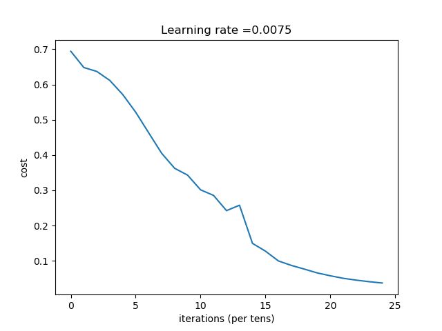
运行后输出的结果是:
Cost after iteration 0: 0.694163741553
Cost after iteration 100: 0.648266362508
Cost after iteration 200: 0.637126344142
Cost after iteration 300: 0.611710351257
.......
Cost after iteration 2100: 0.0505762788807
Cost after iteration 2200: 0.0453126197353
Cost after iteration 2300: 0.0409255847312
Cost after iteration 2400: 0.0372231796013
Accuracy: 1.0
Accuracy: 0.68
其对应的折线图:
L层模型的使用
使用深度神经网络优化参数:
if __name__ == "__main__":
    # 获取数据
    train_x_orig, train_y, test_x_orig, test_y, classes = load_dataset()

    # 重塑培训和测试范例。
    train_x_flatten = train_x_orig.reshape(train_x_orig.shape[0], -1).T
    test_x_flatten = test_x_orig.reshape(test_x_orig.shape[0], -1).T

    # 将数据标准化,使其具有0到1之间的特征值
    train_x = train_x_flatten / 255.
    test_x = test_x_flatten / 255.

    layers_dims_l = [12288, 20, 7, 5, 1]
    parameters = L_layer_model(train_x, train_y, layers_dims_l, num_iterations=2500, print_cost=True)
    pred_train = predict(train_x, train_y, parameters)
    pred_test = predict(test_x, test_y, parameters)
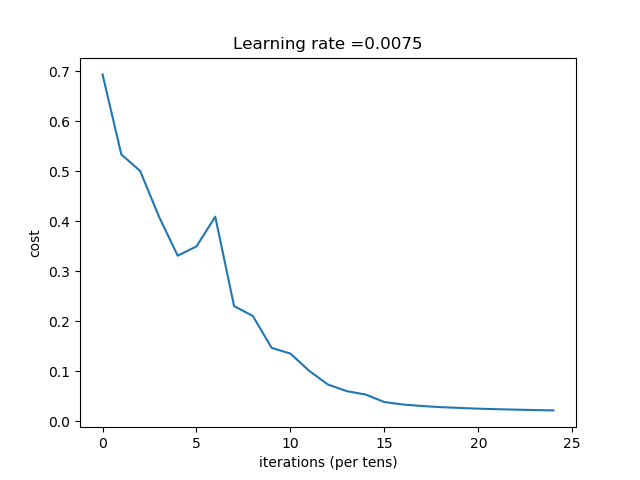
深度神经网络输出的日志如下:
Cost after iteration 0: 0.693828
Cost after iteration 100: 0.533567
Cost after iteration 200: 0.500737
Cost after iteration 300: 0.409495
.....
Cost after iteration 2100: 0.023786
Cost after iteration 2200: 0.022884
Cost after iteration 2300: 0.022056
Cost after iteration 2400: 0.021382
Accuracy: 0.980861244019
Accuracy: 0.7
其对应的折线图如下:
预测自己的图像
训练好的模型也可以用来预测模型自己的图像:
if __name__ == "__main__":
    # 获取数据
    train_x_orig, train_y, test_x_orig, test_y, classes = load_dataset()

    # 重塑培训和测试范例。
    train_x_flatten = train_x_orig.reshape(train_x_orig.shape[0], -1).T
    test_x_flatten = test_x_orig.reshape(test_x_orig.shape[0], -1).T

    # 将数据标准化,使其具有0到1之间的特征值
    train_x = train_x_flatten / 255.
    test_x = test_x_flatten / 255.

    layers_dims_l = [12288, 20, 7, 5, 1]
    parameters = L_layer_model(train_x, train_y, layers_dims_l, num_iterations=2500, print_cost=True)
    infer_image('images/cat2.jpg', parameters, train_x_orig.shape[1])
预测的结果如下:
y = 1.0, your L-layer model predicts a "cat" picture.
参考资料
该笔记是学习吴恩达老师的课程写的。初学者入门,如有理解有误的,欢迎批评指正!