Foreword
CrowdNet is a crowd density estimation model proposed in 2016. Its paper is titled “CrowdNet: A Deep Convolutional Network for DenseCrowd Counting”. The CrowdNet model mainly consists of a deep convolutional neural network and a shallow convolutional neural network. It is trained by inputting the original image and the density map obtained from the Gaussian filter. The final model estimates the number of pedestrians in the image. Of course, this can not only be used for crowd density estimation; theoretically, it should also be applicable to density estimation of other animals, etc.
Project Open Source Address: https://github.com/yeyupiaoling/PaddlePaddle-CrowdNet.git
The development environment for this project is:
- Windows 10
- Python 3.7
- PaddlePaddle 2.0.0a0
Implementation of the CrowdNet Model
The following is the structure diagram of the CrowdNet model. From the diagram, it can be seen that the CrowdNet model is composed of a deep convolutional network (Deep Network) and a shallow convolutional network (Shallow Network). The two networks are concatenated into one network, then input into a convolutional layer with a convolution kernel number and size of 1. Finally, a density map data is obtained through interpolation. The estimated number of people can be obtained by counting this density.
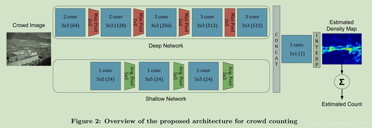
In PaddlePaddle, the following code can be used to implement the above CrowdNet model. Both convolutional layers in the deep convolutional network and shallow convolutional network use the conv_bn convolutional layer, which combines the convolutional layer and batch_norm. In this project, the input image size is [3, 640, 480], and the density map size is [1, 80, 60]. Therefore, the output shape of the deep convolutional network is [512, 80, 60], and the output of the shallow neural network is [24, 80, 60]. The outputs of the two networks are concatenated using the fluid.layers.concat() interface. After concatenation, they are input into fluid.layers.conv2d(), and finally, the fluid.layers.resize_bilinear() bilinear interpolation method is used to output a density map. The final fluid.layers.reduce_sum() is used to facilitate directly outputting the estimated number of people during prediction.
def deep_network(img):
    x = img
    x = conv_bn(input=x, num_filters=64, filter_size=3, padding=1, act='relu')
    x = conv_bn(input=x, num_filters=64, filter_size=3, padding=1, act='relu')
    x = fluid.layers.pool2d(input=x, pool_size=2, pool_stride=2)
    x = fluid.layers.dropout(x=x, dropout_prob=0.25)
    x = conv_bn(input=x, num_filters=128, filter_size=3, padding=1, act='relu')
    x = conv_bn(input=x, num_filters=128, filter_size=3, padding=1, act='relu')
    x = fluid.layers.pool2d(input=x, pool_size=2, pool_stride=2)
    x = fluid.layers.dropout(x=x, dropout_prob=0.25)
    x = conv_bn(input=x, num_filters=256, filter_size=3, padding=1, act='relu')
    x = conv_bn(input=x, num_filters=256, filter_size=3, padding=1, act='relu')
    x = conv_bn(input=x, num_filters=256, filter_size=3, padding=1, act='relu')
    x = fluid.layers.pool2d(input=x, pool_size=2, pool_stride=2)
    x = fluid.layers.dropout(x=x, dropout_prob=0.5)
    x = conv_bn(input=x, num_filters=512, filter_size=3, padding=1, act='relu')
    x = conv_bn(input=x, num_filters=512, filter_size=3, padding=1, act='relu')
    x = conv_bn(input=x, num_filters=512, filter_size=3, padding=1, act='relu')
    x = fluid.layers.pool2d(input=x, pool_size=3, pool_stride=1, pool_padding=1)
    x = conv_bn(input=x, num_filters=512, filter_size=3, padding=1, act='relu')
    x = conv_bn(input=x, num_filters=512, filter_size=3, padding=1, act='relu')
    x = conv_bn(input=x, num_filters=512, filter_size=3, padding=1)
    x = fluid.layers.dropout(x=x, dropout_prob=0.5)
    return x


def shallow_network(img):
    x = img
    x = conv_bn(input=x, num_filters=24, filter_size=5, padding=3, act='relu')
    x = fluid.layers.pool2d(input=x, pool_size=5, pool_type='avg', pool_stride=2)
    x = conv_bn(input=x, num_filters=24, filter_size=5, padding=3, act='relu')
    x = fluid.layers.pool2d(input=x, pool_size=5, pool_type='avg', pool_stride=2)
    x = conv_bn(input=x, num_filters=24, filter_size=5, padding=4, act='relu')
    x = fluid.layers.pool2d(input=x, pool_size=5, pool_type='avg', pool_stride=2)
    return x

# Create CrowdNet network model
net_out1 = deep_network(images)
net_out2 = shallow_network(images)
concat_out = fluid.layers.concat([net_out1, net_out2], axis=1)
conv_end = fluid.layers.conv2d(input=concat_out, num_filters=1, filter_size=1)
# Bilinear interpolation
map_out = fluid.layers.resize_bilinear(conv_end, out_shape=(80, 60))
# Sum to avoid Batch dimension
sum_ = fluid.layers.reduce_sum(map_out, dim=[1, 2, 3])
sum_ = fluid.layers.reshape(sum_, [-1, 1])
The structure of the CrowdNet model implemented through the above code is shown in the following figure:

Training the Model
This project uses a publicly available crowd density dataset from Baidu. The dataset download link is: https://aistudio.baidu.com/aistudio/datasetdetail/1917. After downloading, perform the following operations:
- Place the train.json file in the data directory
- Unzip test_new.zip into the data directory
- Unzip train_new.zip into the data directory
This project provides a script create_list.py that can generate the standard format of the Baidu public dataset into the annotation format required by this project. Executing the script can generate a data list in the following format. If developers want to train their own datasets, they can generate the image annotation data in the following format:
data/train/4c93da45f7dc854a31a4f75b1ee30056.jpg [(171, 200), (365, 144), (306, 155), (451, 204), (436, 252), (600, 235)]
data/train/3a8c1ed636145f23e2c5eafce3863bb2.jpg [(788, 205), (408, 250), (115, 233), (160, 261), (226, 225), (329, 161)]
data/train/075ed038030094f43f5e7b902d41d223.jpg [(892, 646), (826, 763), (845, 75), (896, 260), (773, 752)]
The input label of the model is a density map. The following is a simple introduction to how to generate a density map from annotation data. It is actually generated using Gaussian filters with different kernels, resulting in a density map that is 8 times smaller than the input image.
import json
import numpy as np
import scipy
from PIL import Image
import matplotlib.pyplot as plt
from matplotlib import cm as CM
import scipy
import scipy.spatial
from PIL import Image
from scipy.ndimage.filters import gaussian_filter
import os

# Image preprocessing
def picture_opt(img, ann):
    # Resized image size
    train_img_size = (640, 480)
    gt = []
    size_x, size_y = img.size
    img = img.resize(train_img_size, Image.ANTIALIAS)

    for b_l in range(len(ann)):
        x = ann[b_l][0]
        y = ann[b_l][1]
        x = (x * train_img_size[0] / size_x) / 8
        y = (y * train_img_size[1] / size_y) / 8
        gt.append((x, y))

    img = np.array(img) / 255.0
    return img, gt

# Gaussian filtering
def gaussian_filter_density(gt):
    density = np.zeros(gt.shape, dtype=np.float32)
    gt_count = np.count_nonzero(gt)
    if gt_count == 0:
        return density
    pts = np.array(list(zip(np.nonzero(gt)[1].ravel(), np.nonzero(gt)[0].ravel())))
    tree = scipy.spatial.KDTree(pts.copy(), leafsize=2048)
    distances, locations = tree.query(pts, k=4)
    for i, pt in enumerate(pts):
        pt2d = np.zeros(gt.shape, dtype=np.float32)
        pt2d[pt[1], pt[0]] = 1.
        if gt_count > 1:
            sigma = (distances[i][1] + distances[i][2] + distances[i][3]) * 0.1
        else:
            sigma = np.average(np.array(gt.shape)) / 2. / 2.
        density += scipy.ndimage.filters.gaussian_filter(pt2d, sigma, mode='constant')
    return density


# Density map processing
def ground(img, gt):
    imgs = img
    x = imgs.shape[0] / 8
    y = imgs.shape[1] / 8
    k = np.zeros((int(x), int(y)))
    for i in range(0, len(gt)):
        if int(gt[i][1]) < int(x) and int(gt[i][0]) < int(y):
            k[int(gt[i][1]), int(gt[i][0])] = 1
    img_sum = np.sum(k)
    k = gaussian_filter_density(k)
    return k, img_sum
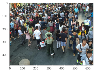
After reading an image and performing scaling preprocessing, the image is not rotated here, but the im.transpose() operation needs to be performed during training to meet the input format of PaddlePaddle.
# Read data list
with open('data/data_list.txt', 'r', encoding='utf-8') as f:
    lines = f.readlines()

line = lines[50]
img_path, gt = line.replace('\n', '').split('\t')
gt = eval(gt)
img = Image.open(img_path)
im, gt = picture_opt(img, gt)

print(im.shape)
plt.imshow(im)
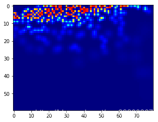
The ground() function is used to generate a density map from the above image. The result of the density map is shown in the following figure. Note that the density map input to PaddlePaddle needs to be rotated because the image data input is rotated, so the density map also needs to be rotated.
k, img_sum = ground(im, gt)
groundtruth = np.asarray(k)
groundtruth = groundtruth.astype('float32')

print("Actual number of people:", img_sum)
print("Density map number of people:", np.sum(groundtruth))
print("Density map size:", groundtruth.shape)

plt.imshow(groundtruth, cmap=CM.jet)
Training Program
The following is the code for train.py. During training, the mean squared error loss function is used, and multiplying the loss value by 6e5 is to prevent the output loss value from being too small.
loss = fluid.layers.square_error_cost(input=map_out, label=label) * 6e5
loss = fluid.layers.mean(loss)
To speed up data reading, an asynchronous data reading method is used, where the next batch of data can be read while training.
py_reader = fluid.io.PyReader(feed_list=[images, label, img_num],
                              capacity=32,
                              iterable=True,
                              return_list=False)
py_reader.decorate_sample_list_generator(paddle.batch(reader.train_reader(data_list_file), batch_size=BATCH_SIZE),
                                         places=fluid.core.CPUPlace())
Before training, add a method to load the pre-trained model. If the model exists, load it and continue training from the previous results.
if PERSISTABLES_MODEL_PATH is not None and os.path.exists(PERSISTABLES_MODEL_PATH):
    def if_exist(var):
        if os.path.exists(os.path.join(PERSISTABLES_MODEL_PATH, var.name)):
            print('loaded: %s' % var.name)
        return os.path.exists(os.path.join(PERSISTABLES_MODEL_PATH, var.name))


    fluid.io.load_vars(exe, PERSISTABLES_MODEL_PATH, main_program=fluid.default_main_program(), predicate=if_exist)
Before executing training, pay attention to the following parameters, which need to be modified according to your actual situation. If the developer follows the above operations, basically no modification is needed, but BATCH_SIZE may need to be adjusted. Because this model is relatively large, if the video memory is small, further adjustments may be required. The following is what the author set in an 8G video memory environment.
# Whether to use GPU
USE_CUDA = True
# Model parameter saving path
PERSISTABLES_MODEL_PATH = 'persistables_model/'
# Prediction model saving path
INFER_MODEL = 'infer_model/'
# Number of training epochs
EPOCHS_SUM = 800
# Batch size
BATCH_SIZE = 6
# Image list path
data_list_file = 'data/data_list.txt'
Finally, execute python train.py to start training the model.
Prediction
By executing infer.py, all images in the data/test/ directory can be predicted, and the results are written to the results.csv file.
The following briefly introduces the prediction process. The prediction model saved during training is loaded to obtain a prediction program.
import matplotlib.pyplot as plt
from matplotlib import cm as CM
import os
import numpy as np
import paddle.fluid as fluid
from PIL import Image

# Whether to use GPU
USE_CUDA = True
INFER_MODEL = 'infer_model/'

place = fluid.CUDAPlace(0) if USE_CUDA else fluid.CPUPlace()
exe = fluid.Executor(place)

[inference_program,
 feed_target_names,
 fetch_targets] = fluid.io.load_inference_model(INFER_MODEL, exe)
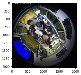
Read an image to be predicted.
image_path = "data/test/00bdc7546131db72333c3e0ac9cf5478.jpg"
test_img = Image.open(image_path)
plt.imshow(test_img)
Preprocess the image by resizing. During prediction, the image is not rotated here, but the transpose() operation is required to meet the input format of PaddlePaddle.
```python
test_img = test_img.resize((640, 480), Image.ANTIALIAS)
test_im = np.array(test_img) / 255.0
test_im = test_im.transpose().reshape(1, 3, 640, 480).astype(‘float32’)