百度機器學習訓練營筆記——數學基礎

均值（mean，average）¶

代表一組數據在分佈上的集中趨勢和總體上的平均水平。
常說的中心化（Zero-Centered）或者零均值化（Mean-subtraction），就是把每個數值都減去均值。

\[\mu=\frac{1}{N}\sum_{i=1}^Nx_i\left(x:x_1,x_2,...,x_N\right)\]

import numpy as np

# 一維數組
x = np.array([-0.02964322, -0.11363636, 0.39417967, -0.06916996, 0.14260276])
print('數據：', x)

# 求均值
avg = np.mean(x)
print('均值：', avg)

輸出：

數據： [-0.02964322 -0.11363636  0.39417967 -0.06916996  0.14260276]
均值： 0.064866578

標準差（Standard Deviation）¶

代表一組數據在分佈上第離散程度。
方差是標準差的平方。

$\(\sigma=\sqrt{\frac{1}{N}\sum_{i=1}^N\left(x_i-\mu\right)^2} \left(x:x_1,x_2,...,x_N\right)$\)

import numpy as np

# 一維數組
x = np.array([-0.02964322, -0.11363636, 0.39417967, -0.06916996, 0.14260276])
print('數據：', x)

# 求標準差
std = np.std(x)
print('標準差：', std)

輸出：

數據： [-0.02964322 -0.11363636  0.39417967 -0.06916996  0.14260276]
標準差： 0.18614576055671836

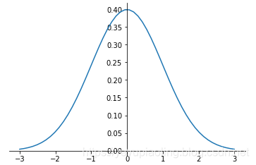
正態分佈（Normal Distribution）¶

又叫“常態分佈”，“高斯分佈”，是最重要的一種分佈。
均值決定位置，方差決定幅度。
表示：$X\sim N\left(\mu,\sigma^2\right)$

正態分佈的概率密度函數：
$\(f(x)=\frac{1}{\sqrt {2\pi\sigma}}e^{-\frac{\left(x-\mu\right)^2}{2\sigma^2}}$\)

import numpy as np
from matplotlib import pyplot as plt

def nd(x, u=-0, d=1):
    return 1/np.sqrt(2*np.pi*d)*np.exp(-(x-u)**2/2/d**2)

x = np.linspace(-3, 3, 50)
y = nd(x)
plt.plot(x, y)

# 調整座標
ax = plt.gca()
ax.spines['right'].set_color('none')
ax.spines['top'].set_color('none')
ax.xaxis.set_ticks_position('bottom')
ax.yaxis.set_ticks_position('left')
ax.spines['bottom'].set_position(('data', 0))
ax.spines['left'].set_position(('data', 0))
plt.show()

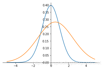
非標準正態分佈的標準化（Normalization）¶

將非標準正態變爲標準正態。
將每個數據減均值，除標準差。

\[y=\frac{x-\mu}{\sigma}\]

import numpy as np
from matplotlib import pyplot as plt

def nd(x, u=0, d=1):
    return 1/np.sqrt(2*np.pi*d)*np.exp(-(x-u)**2/2/d**2)

x = np.linspace(-5, 5, 50)
y1 = nd(x)
y2 = nd(x, 0.5, 2)
plt.plot(x, y1)
plt.plot(x, y2)

# 調整座標
ax = plt.gca()
ax.spines['right'].set_color('none')
ax.spines['top'].set_color('none')
ax.xaxis.set_ticks_position('bottom')
ax.yaxis.set_ticks_position('left')
ax.spines['bottom'].set_position(('data', 0))
ax.spines['left'].set_position(('data', 0))
plt.show()

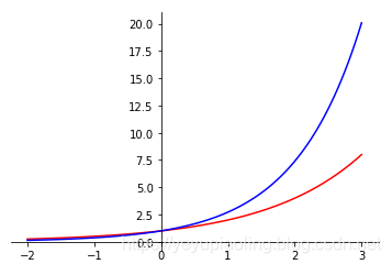
指數函數（Exponent）¶

常用2, e的指數函數；
輸入爲任意實數；
輸出爲非負數。

\[y_1=2^x$$ $$y_2=e^x\]

import numpy as np
from matplotlib import pyplot as plt

x = np.linspace(-2, 3, 100)
y1 = 2**x
y2 = np.exp(x)
plt.plot(x,y1, color='red')
plt.plot(x, y2, color='blue')

# 調整座標
ax = plt.gca()
ax.spines['right'].set_color('none')
ax.spines['top'].set_color('none')
ax.xaxis.set_ticks_position('bottom')
ax.yaxis.set_ticks_position('left')
ax.spines['bottom'].set_position(('data', 0))
ax.spines['left'].set_position(('data', 0))
plt.show()

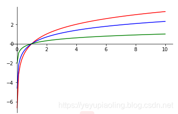
對數函數（Logarithm）¶

常用以2, e, 10爲底的對數函數；
定義域爲正數；
值域爲全體實數；
輸入在(0, 1)範圍內時，輸出爲負數。

$\(y_1=log_2x$\)
$\(y_2=lnx$\)
$\(y_3=lgx$\)

import numpy as np
from matplotlib import pyplot as plt

x = np.linspace(0.01, 10, 100)
y1 = np.log2(x)
y2 = np.log(x)
y3 = np.log10(x)
plt.plot(x, y1, color='red')
plt.plot(x, y2, color='blue')
plt.plot(x, y3, color='green')

# 調整座標
ax = plt.gca()
ax.spines['right'].set_color('none')
ax.spines['top'].set_color('none')
ax.xaxis.set_ticks_position('bottom')
ax.yaxis.set_ticks_position('left')
ax.spines['bottom'].set_position(('data', 0))
ax.spines['left'].set_position(('data', 0))
plt.show()

Softmax函數¶

在分類網絡的輸出層中作激活函數，輸出概率；
先通過指數函數，把所有輸出都變爲整數；
再做歸一化，每個數都除以所有數的和，輸出各分類的概率。

\[P_i=\frac{e^{x_i}}{\sum_{i=1}^Ne^{x_i}}\left(x:x_1,x_2,\ldots,x_N\right)\]

import numpy as np

x = np.array([-0.02964322, -0.11363636, 0.39417967, -0.06916996, 0.14260276])
print('原始輸出：', x)
prob = np.exp(x)/np.sum(np.exp(x))
print('概率輸出：', prob)

輸出：

原始輸出： [-0.02964322 -0.11363636  0.39417967 -0.06916996  0.14260276]
概率輸出： [0.17868493 0.16428964 0.27299323 0.17175986 0.21227234]

One-hot 編碼¶

在分類網絡中，用於對類別進行編碼；
編碼長度等於類別數；
每個編碼只有一位爲1，其餘都爲0；
所有編碼向量都正交。

示例：

假如有5類，則編碼爲：

第一類：[1, 0, 0, 0, 0]

第二類：[0, 1, 0, 0, 0]

第三類：[0, 0, 1, 0, 0]

第四類：[0, 0, 0, 1, 0]

第五類：[0, 0, 0, 0, 1]

交叉熵（Cross Entropy）¶

常用於分類問題中，做損失函數；
從分佈的角度，讓預測概率趨近於標籤。

$Label:[l_1, l_2, \ldots, l_N]$ ——經過One-hot編碼

$predict:[P_1, P_2, \ldots, P_N]$ ——經過Softmax函數

\[ce=-\sum_{i=1}^Nl_i\cdot\log^{P_i}\]

import numpy as np

# one-hot 編碼的標籤
label = np.array([0,0,1,0,0])
print('分類標籤：', label)
# 網絡實際輸出
x1 = np.array([-0.02964322, -0.11363636, 3.39417967, -0.06916996, 0.14260276])
x2 = np.array([-0.02964322, -0.11363636, 1.39417967, -0.06916996, 5.14260276])
print('網絡輸出1:', x1)
print('網絡輸出2:', x2)
# softmax 之後的模擬概率
p1 = np.exp(x1) / np.sum(np.exp(x1))
p2 = np.exp(x2) / np.sum(np.exp(x2))
print('概率輸出1:', p1)
print('概率輸出2:', p2)
# 交叉熵
ce1 = -np.sum(label * np.log(p1))
ce2 = -np.sum(label * np.log(p2))
print('交叉熵1:', ce1)
print('交叉熵2:', ce2)

輸出：

分類標籤： [0 0 1 0 0]
網絡輸出1: [-0.02964322 -0.11363636  3.39417967 -0.06916996  0.14260276]
網絡輸出2: [-0.02964322 -0.11363636  1.39417967 -0.06916996  5.14260276]
概率輸出1: [0.02877271 0.02645471 0.88293386 0.0276576  0.03418112]
概率輸出2: [0.00545423 0.00501482 0.02265122 0.00524284 0.96163688]
交叉熵1: 0.12450498821197674
交叉熵2: 3.787541448750617

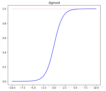
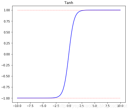
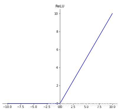
激活函數（Activation Function）¶

引入非線性因素，使模型有更強的表達能力；
輸出層採用softmax激活，可以模擬輸出概率；
sigmoid和tanh都有飽和區，會導致梯度消失；
在深度學習中，sigmoid和tanh主要用於做各種門或開關；
在深度學習中，最常用的激活函數爲ReLU及其變體。

\[\delta(x)=\frac{1}{1+e^{-x}}$$ $$Tanh(x)=\frac{e^x-e^{-x}}{e^x+e^{-x}}$$ $$ReLU(x)=max(x, 0)\]

import numpy as np
from matplotlib import pyplot as plt

x = np.linspace(-10, 10, 100)
# plt.figure(31)
plt.figure(figsize=(10, 20))

# Sigmoid
sigmoid = 1 / (1 + np.exp(-x))
top = np.ones(100)
plt.subplot(311)
plt.plot(x, sigmoid, color='blue')
plt.plot(x, top, color='red', linestyle='-.', linewidth=0.5)
plt.title(s='Sigmoid')

# Tanh
tanh = (np.exp(x) - np.exp(-x)) / (np.exp(x) + np.exp(-x))
top = np.ones(100)
bottom = -np.ones(100)
plt.subplot(312)
plt.plot(x, tanh, color='blue')
plt.plot(x, top, color='red', linestyle='-.', linewidth=0.5)
plt.plot(x, bottom, color='red', linestyle='-.', linewidth=0.5)
plt.title('Tanh')

# ReLU
relu = np.maximum(x, 0)
plt.subplot(313)
plt.plot(x, relu, color='blue')
plt.title('ReLU')


# 調整座標
ax = plt.gca()
ax.spines['right'].set_color('none')
ax.spines['top'].set_color('none')
ax.xaxis.set_ticks_position('bottom')
ax.yaxis.set_ticks_position('left')
ax.spines['bottom'].set_position(('data', 0))
ax.spines['left'].set_position(('data', 0))
plt.show()

源代碼地址：https://aistudio.baidu.com/aistudio/projectdetail/176057