目錄¶

@[toc]

前言¶

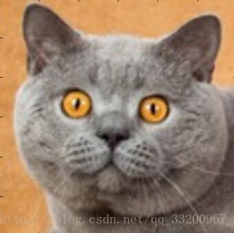
這裏使用到的是一個貓的數據集，根據這個數據集訓練圖像是不是貓，數據集的圖像如下：

導入包¶

如果沒有安裝對應的包，請使用pip安裝對應的包，這個使用了一個lr_utils的工具類，這個工具類是加載數據集的工具，可以到這裏下載。這個工具類也使用一個h5py，所以也要安裝該包。

# coding=utf-8
import matplotlib.pyplot as plt
import numpy as np
import scipy
from scipy import ndimage
from lr_utils import load_dataset

獲取數據¶

接下來就是加載數據和對數據進行處理

# 加載數據
train_set_x_orig, train_set_y, test_set_x_orig, test_set_y, classes = load_dataset()

# 讀取圖像的大小
m_train = train_set_x_orig.shape[0]
m_test = test_set_x_orig.shape[0]
num_px = train_set_x_orig.shape[1]

# 把圖像的(num_px, num_px, 3)大小轉成numpy數據的(num_px ∗ num_px ∗ 3, 1).
train_set_x_flatten = train_set_x_orig.reshape(train_set_x_orig.shape[0], -1).T
test_set_x_flatten = test_set_x_orig.reshape(test_set_x_orig.shape[0], -1).T

# 對數據集進行居中和標準化
train_set_x = train_set_x_flatten / 255.
test_set_x = test_set_x_flatten / 255.

學習算法的一般體系結構¶

定義模型結構(例如輸入特性的數量)
初始化模型的參數
循環:
- 計算當前損失(正向傳播)
- 計算當前梯度(向後傳播)
- 更新參數(梯度下降)

定義模型結構¶

定義sigmoid函數¶

sigmoid函數的公式如下：
$\(sigmoid(x) = \frac{1}{1 + e^{-(x)}}\tag{1}$\)
我們在調用的時候，使用地點參數是$ w^T x + b$，所以計算公式如下：
$\(sigmoid( w^T x + b) = \frac{1}{1 + e^{-(w^T x + b)}}\tag{2}$\)

def sigmoid(x):
    """
    計算sigmoid函數
    :param x: 任意大小的標量或者numpy數組
    :return: sigmoid(x)
    """
    s = 1 / (1 + np.exp(-x))
    return s

定義計算損失值函數¶

通過“正向”和“反向”傳播，計算損失值。
正向傳播:

獲取 X
計算 $A = \sigma(w^T X + b) = (a^{(1)}, a^{(2)}, ..., a^{(m-1)}, a^{(m)})$
計算損失函數: $J = -\frac{1}{m}\sum_{i=1}^{m}y^{(i)}\log(a^{(i)})+(1-y^{(i)})\log(1-a^{(i)})$

計算dw和db使用到的兩條公式:

\[ \frac{\partial J}{\partial w} = \frac{1}{m}X(A-Y)^T\tag{3}$$ $$ \frac{\partial J}{\partial b} = \frac{1}{m} \sum_{i=1}^m (a^{(i)}-y^{(i)})\tag{4}\]

def propagate(w, b, X, Y):
    """
    實現上述傳播的成本函數及其梯度
    :param w: 權重，一個numpy數組大小(num_px * num_px * 3,1)
    :param b: 偏差,一個標量
    :param X: 數據大小(num_px * num_px * 3，例子數量)
    :param Y: 真正的“標籤”向量(包含0如果非貓，1如果貓)的大小(1，例子數量)
    :return: 
    cost -- Logistic迴歸的負對數似然成本。
    dw -- 關於w的損失梯度，與w相同。
    db -- 關於b的損失梯度，與b相同。
    """
    m = X.shape[1]
    A = sigmoid(np.add(np.dot(w.T, X), b))  # compute activation
    cost = -(np.dot(Y, np.log(A).T) + np.dot(1 - Y, np.log(1 - A).T)) / m  # compute cost
    dw = np.dot(X, (A - Y).T) / m
    db = np.sum(A - Y) / m
    assert (dw.shape == w.shape)
    assert (db.dtype == float)
    cost = np.squeeze(cost)
    assert (cost.shape == ())
    grads = {"dw": dw,
             "db": db}

    return grads, cost

初始化模型的參數¶

開始給權重值和偏差初始化一個值，權重是一個矢量，偏差是一個標量。

def initialize_with_zeros(dim):
    """
    這個函數爲w創建一個形狀爲0的向量(dim, 1)，並初始化b爲0。
    :param dim: 我們想要的w向量的大小(或者這個例子中的參數個數)
    :return: 
    w -- 初始形狀矢量(dim, 1)
    b -- 初始化標量(對應於偏差)
    """
    w = np.zeros((dim, 1))
    b = 0
    assert (w.shape == (dim, 1))
    assert (isinstance(b, float) or isinstance(b, int))
    return w, b

定義梯度下降算法¶

通過以下的公式規則來更新參數：
$$ \theta = \theta - \alpha \text{ } d\theta\tag{5}$$

def optimize(w, b, X, Y, num_iterations, learning_rate, print_cost=False):
    """
    該函數通過運行梯度下降算法優化w和b
    :param w: 權重，一個numpy數組大小(num_px * num_px * 3,1)
    :param b: 偏差,一個標量
    :param X: 數據大小 (num_px * num_px * 3, 例子數量)
    :param Y: 真正的“標籤”向量(包含0，如非貓，1如果貓)，形狀(1，例子數量)
    :param num_iterations: 優化循環的迭代次數
    :param learning_rate: 梯度下降更新規則的學習速率
    :param print_cost: 確實每100步就打印一次損失
    :return: 
    params -- 字典中包含權重w和偏差b。
    grads -- 字典中包含權重的梯度和關於成本函數的梯度。
    costs -- 在優化過程中計算的所有成本列表，將用於繪製學習曲線。
    """
    costs = []
    for i in range(num_iterations):
        grads, cost = propagate(w, b, X, Y)
        dw = grads["dw"]
        db = grads["db"]
        w = w - learning_rate * dw
        b = b - learning_rate * db
        if i % 100 == 0:
            costs.append(cost)
        if print_cost and i % 100 == 0:
            print ("Cost after iteration %i: %f" % (i, cost))

    params = {"w": w,
              "b": b}

    grads = {"dw": dw,
             "db": db}

    return params, grads, costs

使用Logistic預測¶

然後通過以下的公式可以得到預測結果：
$\(\hat{Y} = A = \sigma(w^T X + b)\tag{6}$\)
當激活值小於等於0.5時，結果是0，如果激活值大於0.5時，結果是1。

def predict(w, b, X):
    """
    使用學習的邏輯迴歸參數預測標籤是否爲0或1 (w, b)
    :param w: 權重，一個numpy數組大小(num_px * num_px * 3,1)
    :param b: 偏差,一個標量
    :param X: 數據大小 (num_px * num_px * 3, 樣本數量)
    :return: 
    Y_prediction -- 一個包含所有關於X中的例子的所有預測(0/1)的numpy數組(vector)。 
    """
    m = X.shape[1]
    Y_prediction = np.zeros((1, m))
    w = w.reshape(X.shape[0], 1)
    A = sigmoid(np.dot(w.T, X) + b)
    for i in range(A.shape[1]):
        if A[0, i] <= 0.5:
            Y_prediction[0, i] = 0
        else:
            Y_prediction[0, i] = 1
    assert (Y_prediction.shape == (1, m))
    return Y_prediction

將所有功能合併到模型中¶

把剛纔編寫好的函數：初始化函數，優化參數函數和預測函數整合到這個model函數統一處理：

def model(X_train, Y_train, X_test, Y_test, num_iterations=2000, learning_rate=0.5, print_cost=False):
    """
    通過調用之前實現的函數構建邏輯迴歸模型。
    :param X_train: 由形狀的numpy數組表示的訓練集(num_px * num_px * 3, m_train)
    :param Y_train: 由形狀(1,m_train)的numpy陣列(矢量)表示的訓練標籤
    :param X_test: 由形狀的numpy數組表示的測試集(num_px * num_px * 3, m_test)
    :param Y_test: 由形狀(1,m_test)的numpy數組(vector)表示的測試標籤
    :param num_iterations: 表示要優化參數的迭代次數的超參數。
    :param learning_rate: 表示optimize()更新規則中使用的學習速率的超參數
    :param print_cost: 設置爲true，每100次迭代打印成本。
    :return: 
    d -- 包含模型信息的字典。
    """
    w, b = initialize_with_zeros(X_train.shape[0])
    parameters, grads, costs = optimize(w, b, X_train, Y_train, num_iterations, learning_rate, print_cost)

    w = parameters["w"]
    b = parameters["b"]

    Y_prediction_test = predict(w, b, X_test)
    Y_prediction_train = predict(w, b, X_train)

    print("train accuracy: {} %".format(100 - np.mean(np.abs(Y_prediction_train - Y_train)) * 100))
    print("test accuracy: {} %".format(100 - np.mean(np.abs(Y_prediction_test - Y_test)) * 100))

    d = {"costs": costs,
         "Y_prediction_test": Y_prediction_test,
         "Y_prediction_train": Y_prediction_train,
         "w": w,
         "b": b,
         "learning_rate": learning_rate,
         "num_iterations": num_iterations}

    return d

測試各種的學習率對模型收斂的效果¶

嘗試不同的學習率，可以得到最好的訓練效果。學習率決定我們更新參數的速度。如果學習率過高，我們可能會“超過”最優值。同樣，如果它太小，我們將需要太多迭代才能收斂到最佳值，所以一個好的學習率至關重要。

def test_anther_lr():
    learning_rates = [0.01, 0.001, 0.0001]
    models = {}
    for i in learning_rates:
        print ("learning rate is: " + str(i))
        models[str(i)] = model(train_set_x, train_set_y, test_set_x, test_set_y, num_iterations=1500,
                               learning_rate=i, print_cost=False)
        print ('\n' + "-------------------------------------------------------" + '\n')

    for i in learning_rates:
        plt.plot(np.squeeze(models[str(i)]["costs"]), label=str(models[str(i)]["learning_rate"]))

    plt.ylabel('cost')
    plt.xlabel('iterations (hundreds)')

    legend = plt.legend(loc='upper center', shadow=True)
    frame = legend.get_frame()
    frame.set_facecolor('0.90')
    plt.show()

預測自己的圖像¶

通過這個函數，可以是個模型字典的參數就可以獲取預測結果了。通過接收圖像修該成訓練時的圖像大小。要注意的是隻接受JPG格式的圖像。

def infer_mydata(my_image, d):
    """
    預測自己的圖像
    :param my_image: 圖像名字，只接受jpg格式
    :param d: 訓練好的模型信息的字典
    :return: 
    """
    fname = "images/" + my_image
    image = np.array(ndimage.imread(fname, flatten=False))
    my_image = scipy.misc.imresize(image, size=(num_px, num_px)).reshape((1, num_px * num_px * 3)).T
    my_predicted_image = predict(d["w"], d["b"], my_image)

    plt.imshow(image)
    print("y = " + str(np.squeeze(my_predicted_image)) + ", your algorithm predicts a \"" + classes[
        int(np.squeeze(my_predicted_image)),].decode("utf-8") + "\" picture.")

啓動訓練¶

在這裏可以調用model()函數進行訓練模型，獲得訓練後的模型信息的字典，使用這些字典就可以預測圖像了。
通過調用infer_mydata()這個函數就可以預測圖像了，這個要注意的是，圖像只支持JPG格式。
test_anther_lr()函數是使用不用的學習率來觀察不同學習率的收斂情況。

if __name__ == "__main__":
    d = model(train_set_x, train_set_y, test_set_x, test_set_y, num_iterations=1000, learning_rate=0.005,
              print_cost=True)
    # infer_mydata('cat2.jpg', d)
    # test_anther_lr()

輸出結果如下：

Cost after iteration 0: 0.693147
Cost after iteration 100: 0.584508
Cost after iteration 200: 0.466949
Cost after iteration 300: 0.376007
Cost after iteration 400: 0.331463
Cost after iteration 500: 0.303273
Cost after iteration 600: 0.279880
Cost after iteration 700: 0.260042
Cost after iteration 800: 0.242941
Cost after iteration 900: 0.228004
train accuracy: 96.6507177033 %
test accuracy: 72.0 %

全部代碼¶

爲了方便閱讀代碼，筆者把這篇的所有代碼都放出來了：

# coding=utf-8
import matplotlib.pyplot as plt
import numpy as np
import scipy
from scipy import ndimage
from lr_utils import load_dataset

# 加載數據
train_set_x_orig, train_set_y, test_set_x_orig, test_set_y, classes = load_dataset()

# 讀取圖像的大小
m_train = train_set_x_orig.shape[0]
m_test = test_set_x_orig.shape[0]
num_px = train_set_x_orig.shape[1]

# 把圖像的(num_px, num_px, 3)大小轉成numpy數據的(num_px ∗ num_px ∗ 3, 1).
train_set_x_flatten = train_set_x_orig.reshape(train_set_x_orig.shape[0], -1).T
test_set_x_flatten = test_set_x_orig.reshape(test_set_x_orig.shape[0], -1).T

# 對數據集進行居中和標準化
train_set_x = train_set_x_flatten / 255.
test_set_x = test_set_x_flatten / 255.


# 定義sigmoid函數
def sigmoid(x):
    """
    計算sigmoid函數
    :param x: 任意大小的標量或者numpy數組
    :return: sigmoid(x)
    """
    s = 1 / (1 + np.exp(-x))
    return s


# 初始化權重值和偏差
def initialize_with_zeros(dim):
    """
    這個函數爲w創建一個形狀爲0的向量(dim, 1)，並初始化b爲0。
    :param dim: 我們想要的w向量的大小(或者這個例子中的參數個數)
    :return: 
    w -- 初始形狀矢量(dim, 1)
    b -- 初始化標量(對應於偏差)
    """
    w = np.zeros((dim, 1))
    b = 0
    assert (w.shape == (dim, 1))
    assert (isinstance(b, float) or isinstance(b, int))
    return w, b


# 通過正向傳播和反向傳播計算損失值
def propagate(w, b, X, Y):
    """
    實現上述傳播的成本函數及其梯度
    :param w: 權重，一個numpy數組大小(num_px * num_px * 3,1)
    :param b: 偏差,一個標量
    :param X: 數據大小(num_px * num_px * 3，例子數量)
    :param Y: 真正的“標籤”向量(包含0如果非貓，1如果貓)的大小(1，例子數量)
    :return: 
    cost -- Logistic迴歸的負對數似然成本。
    dw -- 關於w的損失梯度，與w相同。
    db -- 關於b的損失梯度，與b相同。
    """
    m = X.shape[1]
    A = sigmoid(np.add(np.dot(w.T, X), b))  # compute activation
    cost = -(np.dot(Y, np.log(A).T) + np.dot(1 - Y, np.log(1 - A).T)) / m  # compute cost
    dw = np.dot(X, (A - Y).T) / m
    db = np.sum(A - Y) / m
    assert (dw.shape == w.shape)
    assert (db.dtype == float)
    cost = np.squeeze(cost)
    assert (cost.shape == ())
    grads = {"dw": dw,
             "db": db}

    return grads, cost


# 通過梯度下降算法來優化w和b
def optimize(w, b, X, Y, num_iterations, learning_rate, print_cost=False):
    """
    該函數通過運行梯度下降算法優化w和b
    :param w: 權重，一個numpy數組大小(num_px * num_px * 3,1)
    :param b: 偏差,一個標量
    :param X: 數據大小 (num_px * num_px * 3, 例子數量)
    :param Y: 真正的“標籤”向量(包含0，如非貓，1如果貓)，形狀(1，例子數量)
    :param num_iterations: 優化循環的迭代次數
    :param learning_rate: 梯度下降更新規則的學習速率
    :param print_cost: 確實每100步就打印一次損失
    :return: 
    params -- 字典中包含權重w和偏差b。
    grads -- 字典中包含權重的梯度和關於成本函數的梯度。
    costs -- 在優化過程中計算的所有成本列表，將用於繪製學習曲線。
    """
    costs = []
    for i in range(num_iterations):
        grads, cost = propagate(w, b, X, Y)
        dw = grads["dw"]
        db = grads["db"]
        w = w - learning_rate * dw
        b = b - learning_rate * db
        if i % 100 == 0:
            costs.append(cost)
        if print_cost and i % 100 == 0:
            print ("Cost after iteration %i: %f" % (i, cost))

    params = {"w": w,
              "b": b}

    grads = {"dw": dw,
             "db": db}

    return params, grads, costs


# 使用Logistic預測
def predict(w, b, X):
    """
    使用學習的邏輯迴歸參數預測標籤是否爲0或1 (w, b)
    :param w: 權重，一個numpy數組大小(num_px * num_px * 3,1)
    :param b: 偏差,一個標量
    :param X: 數據大小 (num_px * num_px * 3, 樣本數量)
    :return: 
    Y_prediction -- 一個包含所有關於X中的例子的所有預測(0/1)的numpy數組(vector)。 
    """
    m = X.shape[1]
    Y_prediction = np.zeros((1, m))
    w = w.reshape(X.shape[0], 1)
    A = sigmoid(np.dot(w.T, X) + b)
    for i in range(A.shape[1]):
        if A[0, i] <= 0.5:
            Y_prediction[0, i] = 0
        else:
            Y_prediction[0, i] = 1
    assert (Y_prediction.shape == (1, m))
    return Y_prediction


# 將所有功能合併到模型中
def model(X_train, Y_train, X_test, Y_test, num_iterations=2000, learning_rate=0.5, print_cost=False):
    """
    通過調用之前實現的函數構建邏輯迴歸模型。
    :param X_train: 由形狀的numpy數組表示的訓練集(num_px * num_px * 3, m_train)
    :param Y_train: 由形狀(1,m_train)的numpy陣列(矢量)表示的訓練標籤
    :param X_test: 由形狀的numpy數組表示的測試集(num_px * num_px * 3, m_test)
    :param Y_test: 由形狀(1,m_test)的numpy數組(vector)表示的測試標籤
    :param num_iterations: 表示要優化參數的迭代次數的超參數。
    :param learning_rate: 表示optimize()更新規則中使用的學習速率的超參數
    :param print_cost: 設置爲true，每100次迭代打印成本。
    :return: 
    d -- 包含模型信息的字典。
    """
    w, b = initialize_with_zeros(X_train.shape[0])
    parameters, grads, costs = optimize(w, b, X_train, Y_train, num_iterations, learning_rate, print_cost)

    w = parameters["w"]
    b = parameters["b"]

    Y_prediction_test = predict(w, b, X_test)
    Y_prediction_train = predict(w, b, X_train)

    print("train accuracy: {} %".format(100 - np.mean(np.abs(Y_prediction_train - Y_train)) * 100))
    print("test accuracy: {} %".format(100 - np.mean(np.abs(Y_prediction_test - Y_test)) * 100))

    d = {"costs": costs,
         "Y_prediction_test": Y_prediction_test,
         "Y_prediction_train": Y_prediction_train,
         "w": w,
         "b": b,
         "learning_rate": learning_rate,
         "num_iterations": num_iterations}

    return d


# 測試各種的學習率對模型收斂的效果
def test_anther_lr():
    learning_rates = [0.01, 0.001, 0.0001]
    models = {}
    for i in learning_rates:
        print ("learning rate is: " + str(i))
        models[str(i)] = model(train_set_x, train_set_y, test_set_x, test_set_y, num_iterations=1500,
                               learning_rate=i, print_cost=False)
        print ('\n' + "-------------------------------------------------------" + '\n')

    for i in learning_rates:
        plt.plot(np.squeeze(models[str(i)]["costs"]), label=str(models[str(i)]["learning_rate"]))

    plt.ylabel('cost')
    plt.xlabel('iterations (hundreds)')

    legend = plt.legend(loc='upper center', shadow=True)
    frame = legend.get_frame()
    frame.set_facecolor('0.90')
    plt.show()


# 預測自己的圖像
def infer_mydata(my_image, d):
    """
    預測自己的圖像
    :param my_image: 圖像名字，只接受jpg格式
    :param d: 訓練好的模型信息的字典
    :return: 
    """
    fname = "images/" + my_image
    image = np.array(ndimage.imread(fname, flatten=False))
    my_image = scipy.misc.imresize(image, size=(num_px, num_px)).reshape((1, num_px * num_px * 3)).T
    my_predicted_image = predict(d["w"], d["b"], my_image)

    plt.imshow(image)
    print("y = " + str(np.squeeze(my_predicted_image)) + ", your algorithm predicts a \"" + classes[
        int(np.squeeze(my_predicted_image)),].decode("utf-8") + "\" picture.")


if __name__ == "__main__":
    d = model(train_set_x, train_set_y, test_set_x, test_set_y, num_iterations=1000, learning_rate=0.005,
              print_cost=True)
    # infer_mydata('cat2.jpg', d)
    # test_anther_lr()

參考資料¶

http://deeplearning.ai/

該筆記是學習吳恩達老師的課程寫的。初學者入門，如有理解有誤的，歡迎批評指正！

目錄¶

前言¶