Table of Contents¶

@[toc]

Introduction¶

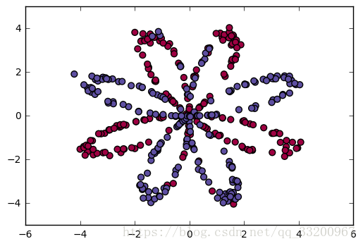
The dataset consists of a red and blue distribution. Its distribution chart is as follows:

Importing Packages¶

Import the required dependent packages. These two are utility functions for loading data and the dataset itself. These programs can be downloaded from here. The utility function uses the sklearn package, which needs to be installed with pip before use.

from planar_utils import sigmoid, load_planar_dataset
from testCases_v2 import *

Loading Data¶

Load the data and obtain its shape

# Load the data
X, Y = load_planar_dataset()

# Get the shape of the data
shape_X = X.shape
shape_Y = Y.shape
m = shape_X[1]

Neural Network Model¶

Defining the Neural Network Structure¶

Define the neural network structure, such as the size of the data, corresponding labels, and the number of hidden layers.

def layer_sizes(X, Y):
    """
    Define the neural network structure
    :param X: Input dataset shape (input size, number of examples)
    :param Y: Label shape (output size, number of examples)
    :return: 
    n_x -- Size of input layer.
    n_h -- Size of hidden layer.
    n_y -- Size of output layer.
    """
    n_x = X.shape[0]
    n_h = 4
    n_y = Y.shape[0]
    return (n_x, n_h, n_y)

Initializing Model Parameters¶

Initialize the model weights and bias values based on the neural network structure, and store the weights and biases in a parameter dictionary. The weight vector uses random initialization, and the bias vector is initialized to a zero matrix.

def initialize_parameters(n_x, n_h, n_y):
    """
    Initialize model parameters
    :param n_x: Size of input layer
    :param n_h: Size of hidden layer
    :param n_y: Size of output layer
    :return: 
    params -- Python dictionary containing your parameters:
                W1 -- Weight matrix shape (n_h, n_x)
                b1 -- Bias vector shape (n_h, 1)
                W2 -- Weight matrix shape (n_y, n_h)
                b2 -- Bias vector shape (n_y, 1)
    """
    np.random.seed(2)

    W1 = np.random.randn(n_h, n_x) * 0.01
    b1 = np.zeros((n_h, 1))
    W2 = np.random.randn(n_y, n_h) * 0.01
    b2 = np.zeros((n_y, 1))

    assert (W1.shape == (n_h, n_x))
    assert (b1.shape == (n_h, 1))
    assert (W2.shape == (n_y, n_h))
    assert (b2.shape == (n_y, 1))

    parameters = {"W1": W1,
                  "b1": b1,
                  "W2": W2,
                  "b2": b2}

    return parameters

Forward Propagation¶

This forward propagation uses two activation functions: tanh and sigmoid.

def forward_propagation(X, parameters):
    """
    Forward propagation
    :param X: Input data size (n_x, m)
    :param parameters: Python dictionary containing parameters (output of initialization function)
    :return: 
    A2 -- Sigmoid output of the second activation.
    cache -- Dictionary containing "Z1", "A1", "Z2", "A2"
    """
    W1 = parameters["W1"]
    b1 = parameters["b1"]
    W2 = parameters["W2"]
    b2 = parameters["b2"]

    Z1 = np.dot(W1, X) + b1
    A1 = np.tanh(Z1)
    Z2 = np.dot(W2, A1) + b2
    A2 = sigmoid(Z2)

    assert (A2.shape == (1, X.shape[1]))

    cache = {"Z1": Z1,
             "A1": A1,
             "Z2": Z2,
             "A2": A2}

    return A2, cache

Calculating the Loss Function¶

The following is the formula for the loss function to be calculated:
$\(J = - \frac{1}{m} \sum\limits_{i = 0}^{m} \large{(} \small y^{(i)}\log\left(a^{[2] (i)}\right) + (1-y^{(i)})\log\left(1- a^{[2] (i)}\right) \large{)} \small\tag{1}$\)

def compute_cost(A2, Y):
    """
    Calculate cross-entropy cost as per equation (1)
    :param A2: Sigmoid output of the second activation, shape (1, number of examples)
    :param Y: "True" label vector shape (1, number of samples)
    :return: 
    cost -- Cross-entropy cost from equation (1)
    """
    m = Y.shape[1]  # number of examples

    logprobs = np.multiply(np.log(A2), Y) + np.multiply(1 - Y, np.log(1 - A2))
    cost = -(np.sum(logprobs)) / m

    cost = np.squeeze(cost)  # Ensure cost is the expected dimension.
    assert (isinstance(cost, float))

    return cost

Backward Propagation¶

Backward propagation uses the following formulas:

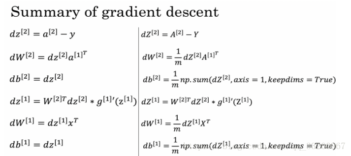
def backward_propagation(parameters, cache, X, Y):
    """
    Implement backward propagation using the instructions above.
    :param parameters: Python dictionary containing our parameters.
    :param cache: Python dictionary containing "Z1", "A1", "Z2", "A2".
    :param X: Input data shape (2, number of examples)
    :param Y: "True" label vector shape (1, number of samples)
    :return: 
    grads -- Python dictionary containing gradients for each parameter
    """
    m = X.shape[1]
    m = float(m)

    W1 = parameters["W1"]
    W2 = parameters["W2"]

    A1 = cache["A1"]
    A2 = cache["A2"]

    dZ2 = A2 - Y
    dW2 = (1 / m) * np.dot(dZ2, A1.T)
    db2 = (1 / m) * np.sum(dZ2, axis=1, keepdims=True)
    dZ1 = np.dot(W2.T, dZ2) * (1 - np.power(A1, 2))
    dW1 = (1 / m) * np.dot(dZ1, X.T)
    db1 = (1 / m) * np.sum(dZ1, axis=1, keepdims=True)

    grads = {"dW1": dW1,
             "db1": db1,
             "dW2": dW2,
             "db2": db2}
    return grads

Updating Parameters¶

Implement the update rule. Use gradient descent. You must use (dW1, db1, dW2, db2) to update (W1, b1, W2, b2) using the update rule formula:
$$ \theta = \theta - \alpha \frac{\partial J }{ \partial \theta }\tag{2}$$

def update_parameters(parameters, grads, learning_rate=1.2):
    """
    Update parameters using the gradient descent update rule given above.
    :param parameters: Python dictionary containing parameters.
    :param grads: Python dictionary containing gradients.
    :param learning_rate: Learning rate
    :return: 
    parameters -- Python dictionary containing updated parameters.
    """
    W1 = parameters["W1"]
    b1 = parameters["b1"]
    W2 = parameters["W2"]
    b2 = parameters["b2"]

    dW1 = grads["dW1"]
    db1 = grads["db1"]
    dW2 = grads["dW2"]
    db2 = grads["db2"]

    W1 = W1 - learning_rate * dW1
    b1 = b1 - learning_rate * db1
    W2 = W2 - learning_rate * dW2
    b2 = b2 - learning_rate * db2

    parameters = {"W1": W1,
                  "b1": b1,
                  "W2": W2,
                  "b2": b2}

    return parameters

Integrating the Model Function¶

Integrate the functions defined above into this function to form a complete neural network.

def nn_model(X, Y, n_h, num_iterations=10000, print_cost=False):
    """
    Integrate the above-defined neural network into this function
    :param X: Dataset shape (2, number of samples)
    :param Y: Label shape (1, number of samples)
    :param n_h: Size of hidden layer
    :param num_iterations: Number of iterations in gradient descent loop.
    :param print_cost: If True, print the cost every 1000 iterations.
    :return: 
    parameters -- Parameters learned by the model. They can be used for prediction.
    """
    np.random.seed(3)
    n_x = layer_sizes(X, Y)[0]
    n_y = layer_sizes(X, Y)[2]

    parameters = initialize_parameters(n_x, n_h, n_y)

    for i in range(0, num_iterations):
        A2, cache = forward_propagation(X, parameters)
        cost = compute_cost(A2, Y)
        grads = backward_propagation(parameters, cache, X, Y)
        parameters = update_parameters(parameters, grads)
        if print_cost and i % 1000 == 0:
            print ("Cost after iteration %i: %f" % (i, cost))

    return parameters

Making Predictions¶

Use your model to make predictions by constructing the predict() function. Use forward propagation to predict results.
$\(y_{prediction} = \mathbb{1} \text{{activation > 0.5}} = \begin{cases} 1 & \text{if}\ activation > 0.5 \\ 0 & \text{otherwise} \end{cases}\tag{3}$\)

def predict(parameters, X):
    """
    Use learned parameters to predict a class for each example in X.
    :param parameters: Python dictionary containing parameters.
    :param X: Input data size (n_x, m)
    :return: 
    predictions -- Model prediction vector (red:0 / blue: 1)
    """
    A2, cache = forward_propagation(X, parameters)
    predictions = A2 > 0.5
    return predictions

Testing Different Hidden Layers¶

By testing different numbers of hidden layers, observe the model’s prediction performance and obtain the optimal number of hidden layers.

def test_another_hidden():
    """
    Train with different hidden layers
    :return: 
    """
    hidden_layer_sizes = [1, 2, 3, 4, 5, 20, 50]
    for i, n_h in enumerate(hidden_layer_sizes):
        parameters = nn_model(X, Y, n_h, num_iterations=1000)
        predictions = predict(parameters, X)
        accuracy = float((np.dot(Y, predictions.T) + np.dot(1 - Y, 1 - predictions.T)) / float(Y.size) * 100)
        print ("Accuracy for {} hidden units: {} %".format(n_h, accuracy))

Calling the Function to Train¶

By calling the integrated neural network function nn_model(), train the parameters. After obtaining the parameters, you can use the parameters to predict the data.

if __name__ == "__main__":
    parameters = nn_model(X, Y, n_h=4, num_iterations=10000, print_cost=True)
    predictions = predict(parameters, X)
    print('Accuracy: %d' % float(
        (np.dot(Y, predictions.T) + np.dot(1 - Y, 1 - predictions.T)) / float(Y.size) * 100) + '%')

Training and prediction output results are:

Cost after iteration 0: 0.693048
Cost after iteration 1000: 0.288083
Cost after iteration 2000: 0.254385
Cost after iteration 3000: 0.233864
Cost after iteration 4000: 0.226792
Cost after iteration 5000: 0.222644
Cost after iteration 6000: 0.219731
Cost after iteration 7000: 0.217504
Cost after iteration 8000: 0.219415
Cost after iteration 9000: 0.218547
Accuracy: 90%

This uses different hidden layers for training and prediction

if __name__ == "__main__":
    test_another_hidden()

The following are the different accuracies obtained after training with different hidden layers:

Accuracy for 1 hidden units: 67.75 %
Accuracy for 2 hidden units: 65.25 %
Accuracy for 3 hidden units: 89.5 %
Accuracy for 4 hidden units: 89.25 %
Accuracy for 5 hidden units: 89.5 %
Accuracy for 20 hidden units: 88.0 %
Accuracy for 50 hidden units: 88.0 %

Complete Code¶

For the convenience of readers to read the code, all the code (excluding the two utility classes) is provided here:
```python

coding=utf-8¶

from planar_utils import sigmoid, load_planar_dataset
from testCases_v2 import *

Load the data¶

X, Y = load_planar_dataset()

Get the shape of the data¶

shape_X = X.shape
shape_Y = Y.shape
m = shape_X[1]

def layer_sizes(X, Y):
“”“
Define the neural network structure
:param X: Input dataset shape (input size, number of examples)
:param Y: Label shape (output size, number of examples)
:return:
n_x – Size of input layer.
n_h – Size of hidden layer.
n_y – Size of output layer.
“”“
n_x = X.shape[0]
n_h = 4
n_y = Y.shape[0]
return (n_x, n_h, n_y)

def initialize_parameters(n_x, n_h, n_y):
“”“
Initialize model parameters
:param n_x: Size of input layer
:param n_h: Size of hidden layer
:param n_y: Size of output layer
:return:
params – Python dictionary containing your parameters:
W1 – Weight matrix shape (n_h, n_x)
b1 – Bias vector shape (n_h, 1)
W2 – Weight matrix shape (n_y, n_h)
b2 – Bias vector shape (n_y, 1)
“”“
np.random.seed(2)

W1 = np.random.randn(n_h, n_x) * 0.01
b1 = np.zeros((n_h, 1))
W2 = np.random.randn(n_y, n_h) * 0.01
b2 = np.zeros((n_y, 1))

assert (W1.shape == (n_h, n_x))
assert (b1.shape == (n_h, 1))
assert (W2.shape == (n_y, n_h))
assert (b2.shape == (n_y, 1))

parameters = {"W1": W1,
              "b1": b1,
              "W2": W2,
              "b2": b2}

return parameters

def forward_propagation(X, parameters):
“”“
Forward propagation
:param X: Input data size (n_x, m)
:param parameters: Python dictionary containing parameters (output of initialization function)
:return:
A2 – Sigmoid output of the second activation.
cache – Dictionary containing “Z1”, “A1”, “Z2”, “A2”
“”“
W1 = parameters[“W1”]
b1 = parameters[“b1”]
W2 = parameters[“W2”]
b2 = parameters[“b2”]

Z1 = np.dot(W1, X) + b1
A1 = np.tanh(Z1)
Z2 = np.dot(W2, A1) + b2
A2 = sigmoid(Z