Preface
A team from Minzu University of China, namely Jushen Artificial Intelligence Technology, has publicly released a TibetanMNIST dataset, which is a dataset of Tibetan numerals, on the Kesci website. The original images of the TibetanMNIST dataset are black-and-white images with a size of 350*350. The first digit in the image file name serves as the image label. For example, the image 0_10_398.jpg represents the Tibetan numeral 0. In this project, we will use the convolutional neural network learned in Chapter 4 to complete the classification and recognition of the TibetanMNIST dataset.
Import Required Packages
We mainly use the PaddlePaddle’s fluid and paddle dependency libraries. The cpu_count library is used to obtain the number of current CPUs, and matplotlib is used for displaying images.
import paddle.fluid as fluid
import paddle
import numpy as np
from PIL import Image
import os
from multiprocessing import cpu_count
import matplotlib.pyplot as plt
Generate Image List
Since the TibetanMNIST dataset has been published on the Kesci website, we need to download it from Kesci before creating the project. The dataset title is 【首发活动】TibetanMNIST藏文手写数字数据集. After downloading, you will get a TibetanMnist (350x350) folder containing the original image files. Compress this folder into a zip format and upload it to the AI Studio platform as a personal dataset. Then, when creating the project, you can mount this dataset.
After mounting the dataset, execute the unzip command to obtain a directory TibetanMnist (350x350), where the original image files are stored. You can read all image files in this directory.
!unzip -q /home/aistudio/data/data2134/TibetanMnist(350x350).zip
data_path = './TibetanMnist(350x350)'
data_imgs = os.listdir(data_path)
After obtaining all image paths, we generate an image list file that includes the absolute path of the image and the corresponding label, separated by a tab. The format is as follows, where a label.txt text file should be ignored to avoid errors during reading.
/home/kesci/input/TibetanMNIST5610/TibetanMNIST/TibetanMNIST/8_2_1.jpg  8
/home/kesci/input/TibetanMNIST5610/TibetanMNIST/TibetanMNIST/0_11_264.jpg   0
/home/kesci/input/TibetanMNIST5610/TibetanMNIST/TibetanMNIST/0_13_320.jpg   0
/home/kesci/input/TibetanMNIST5610/TibetanMNIST/TibetanMNIST/3_16_193.jpg   3
with open('./train_data.list', 'w') as f_train:
    with open('./test_data.list', 'w') as f_test:
        for i in range(len(data_imgs)):
            if data_imgs[i] == 'label.txt':
                continue
            if i % 10 == 0:
                f_test.write(os.path.join(data_path, data_imgs[i]) + "\t" + data_imgs[i][0:1] + '\n')
            else:
                f_train.write(os.path.join(data_path, data_imgs[i]) + "\t" + data_imgs[i][0:1] + '\n')
        print('Image list generated.')
Define Data Reading
PaddlePaddle reads training and test data through readers, so we need to define a custom reader. First, we define a train_mapper() function, which preprocesses the image, such as compressing, cropping, and grayscale conversion using the paddle.dataset.image.simple_transform interface. When the parameter is_train is True, it will randomly crop; otherwise, it will center-crop. Generally, testing and prediction use center-cropping. The train_r() function reads image paths and labels from the image list generated in the previous step and passes the image paths to the train_mapper() function for preprocessing. The same operations apply to test data.
def train_mapper(sample):
    img, label = sample
    img = paddle.dataset.image.load_image(file=img, is_color=False)
    img = paddle.dataset.image.simple_transform(im=img, resize_size=32, crop_size=28, is_color=False, is_train=True)
    img = img.flatten().astype('float32') / 255.0
    return img, label

def train_r(train_list_path):
    def reader():
        with open(train_list_path, 'r') as f:
            lines = f.readlines()
            del lines[len(lines)-1]
            for line in lines:
                img, label = line.split('\t')
                yield img, int(label)
    return paddle.reader.xmap_readers(train_mapper, reader, cpu_count(), 1024)

def test_mapper(sample):
    img, label = sample
    img = paddle.dataset.image.load_image(file=img, is_color=False)
    img = paddle.dataset.image.simple_transform(im=img, resize_size=32, crop_size=28, is_color=False, is_train=False)
    img = img.flatten().astype('float32') / 255.0
    return img, label

def test_r(test_list_path):
    def reader():
        with open(test_list_path, 'r') as f:
            lines = f.readlines()
            for line in lines:
                img, label = line.split('\t')
                yield img, int(label)
    return paddle.reader.xmap_readers(test_mapper, reader, cpu_count(), 1024)
Define Convolutional Neural Network
Here, we define a convolutional neural network. You can modify or replace it with other convolutional neural networks as needed.
def cnn(ipt):
    conv1 = fluid.layers.conv2d(input=ipt,
                                num_filters=32,
                                filter_size=3,
                                padding=1,
                                stride=1,
                                name='conv1',
                                act='relu')

    pool1 = fluid.layers.pool2d(input=conv1,
                                pool_size=2,
                                pool_stride=2,
                                pool_type='max',
                                name='pool1')

    bn1 = fluid.layers.batch_norm(input=pool1, name='bn1')

    conv2 = fluid.layers.conv2d(input=bn1,
                                num_filters=64,
                                filter_size=3,
                                padding=1,
                                stride=1,
                                name='conv2',
                                act='relu')

    pool2 = fluid.layers.pool2d(input=conv2,
                                pool_size=2,
                                pool_stride=2,
                                pool_type='max',
                                name='pool2')

    bn2 = fluid.layers.batch_norm(input=pool2, name='bn2')

    fc1 = fluid.layers.fc(input=bn2, size=1024, act='relu', name='fc1')

    fc2 = fluid.layers.fc(input=fc1, size=10, act='softmax', name='fc2')

    return fc2
Get Network
The convolutional neural network defined above is used to obtain a classifier. The input layer is defined through the fluid.layers.data interface, with a shape of [1, 28, 28], representing a grayscale image with a single channel and a width and height of 28.
image = fluid.layers.data(name='image', shape=[1, 28, 28], dtype='float32')
net = cnn(image)
Define Loss Function
Here, the cross-entropy loss function fluid.layers.cross_entropy is used, along with the fluid.layers.accuracy interface to facilitate outputting the average value during training and testing.
label = fluid.layers.data(name='label', shape=[1], dtype='int64')
cost = fluid.layers.cross_entropy(input=net, label=label)
avg_cost = fluid.layers.mean(x=cost)
acc = fluid.layers.accuracy(input=net, label=label, k=1)
Clone Test Program
After defining the loss function and before defining the optimization method, a test program is cloned from the main program.
test_program = fluid.default_main_program().clone(for_test=True)
Define Optimization Method
Next, the optimization method is defined. Here, the Adam optimization method is used; other optimization methods can also be used.
optimizer = fluid.optimizer.AdamOptimizer(learning_rate=0.001)
opt = optimizer.minimize(avg_cost)
Create Executor
Here, the executor is created and specified to use the CPU for training.
place = fluid.CPUPlace()
exe = fluid.Executor(place=place)
exe.run(program=fluid.default_startup_program())
Generate Reader for Image Data
The readers defined above are used to obtain the reader for each batch of data according to the set size.
train_reader = paddle.batch(reader=paddle.reader.shuffle(reader=train_r('./train_data.list'), buf_size=3000), batch_size=128)
test_reader = paddle.batch(reader=test_r('./test_data.list'), batch_size=128)
Define Input Data Dimensions
Define the dimensions of the input data, the first is the image data, and the second is the label corresponding to the image.
feeder = fluid.DataFeeder(place=place, feed_list=[image, label])
Start Training
Start executing the training. Here, only 10 passes are trained; you can set it arbitrarily. After each pass of training, the test dataset is used to test the model’s accuracy and predict the model once.
for pass_id in range(2):
    for batch_id, data in enumerate(train_reader()):
        train_cost, train_acc = exe.run(program=fluid.default_main_program(),
                                        feed=feeder.feed(data),
                                        fetch_list=[avg_cost, acc])
        if batch_id % 100 == 0:
            print('\nPass:%d, Batch:%d, Cost:%f, Accuracy:%f' % (pass_id, batch_id, train_cost[0], train_acc[0]))
        else:
            print('.', end="")

    test_costs = []
    test_accs = []
    for batch_id, data in enumerate(test_reader()):
        test_cost, test_acc = exe.run(program=test_program,
                                      feed=feeder.feed(data),
                                      fetch_list=[avg_cost, acc])
        test_costs.append(test_cost[0])
        test_accs.append(test_acc[0])
    test_cost = sum(test_costs) / len(test_costs)
    test_acc = sum(test_accs) / len(test_accs)
    print('\nTest:%d, Cost:%f, Accuracy:%f' % (pass_id, test_cost, test_acc))

    fluid.io.save_inference_model(dirname='./model', feeded_var_names=['image'], target_vars=[net], executor=exe)
Output information:
Pass:0, Batch:0, Cost:2.971555, Accuracy:0.101562
...................................................................................................
Pass:0, Batch:100, Cost:0.509201, Accuracy:0.859375
........................
Test:0, Cost:0.255964, Accuracy:0.928092

Pass:1, Batch:0, Cost:0.383406, Accuracy:0.882812
...................................................................................................
Pass:1, Batch:100, Cost:0.262583, Accuracy:0.906250
........................
Test:1, Cost:0.210227, Accuracy:0.942152

Pass:2, Batch:0, Cost:0.248821, Accuracy:0.921875
...................................................................................................
Pass:2, Batch:100, Cost:0.121569, Accuracy:0.953125
........................
Test:2, Cost:0.147000, Accuracy:0.959041

Pass:3, Batch:0, Cost:0.219034, Accuracy:0.914062
...................................................................................................
Pass:3, Batch:100, Cost:0.149375, Accuracy:0.929688
........................
Test:3, Cost:0.135075, Accuracy:0.967970

Pass:4, Batch:0, Cost:0.097395, Accuracy:0.960938
...................................................................................................
Pass:4, Batch:100, Cost:0.088472, Accuracy:0.976562
........................
Test:4, Cost:0.130905, Accuracy:0.965254

Pass:5, Batch:0, Cost:0.115069, Accuracy:0.960938
...................................................................................................
Pass:5, Batch:100, Cost:0.132130, Accuracy:0.953125
........................
Test:5, Cost:0.123031, Accuracy:0.969086

Pass:6, Batch:0, Cost:0.083716, Accuracy:0.984375
...................................................................................................
Pass:6, Batch:100, Cost:0.093365, Accuracy:0.968750
........................
Test:6, Cost:0.113957, Accuracy:0.970686

Pass:7, Batch:0, Cost:0.062250, Accuracy:0.976562
...................................................................................................
Pass:7, Batch:100, Cost:0.095572, Accuracy:0.968750
........................
Test:7, Cost:0.097893, Accuracy:0.974182

Pass:8, Batch:0, Cost:0.122696, Accuracy:0.960938
...................................................................................................
Pass:8, Batch:100, Cost:0.154212, Accuracy:0.976562
........................
Test:8, Cost:0.095770, Accuracy:0.969570

Pass:9, Batch:0, Cost:0.105826, Accuracy:0.960938
...................................................................................................
Pass:9, Batch:100, Cost:0.125963, Accuracy:0.976562
........................
Test:9, Cost:0.078607, Accuracy:0.973550
Get Prediction Program
Through the saved prediction model above, a prediction program can be generated for image prediction.
[infer_program, feeded_var_names, target_vars] = fluid.io.load_inference_model(dirname='./model', executor=exe)
Preprocess Data
Before predicting the image, preprocessing of the image is also required.
def load_image(path):
    img = paddle.dataset.image.load_image(file=path, is_color=False)
    img = paddle.dataset.image.simple_transform(im=img, resize_size=32, crop_size=28, is_color=False, is_train=False)
    img = img.astype('float32')
    img = img[np.newaxis, ] / 255.0
    return img
Get Prediction Image
Then, the preprocessed images are added to the list, and multiple images can be predicted together. Then converted to numpy type.
infer_imgs = []
infer_imgs.append(load_image('./TibetanMnist(350x350)/0_10_398.jpg'))
infer_imgs = np.array(infer_imgs)
infer_imgs.shape
Execute Prediction
Finally, execute the prediction. The input data is passed through the feed parameter, and the prediction result is obtained, which is the probability of each category.
result = exe.run(program=infer_program,
                 feed={feeded_var_names[0]:infer_imgs},
                 fetch_list=target_vars)
Parse Results to Get the Label with Maximum Probability
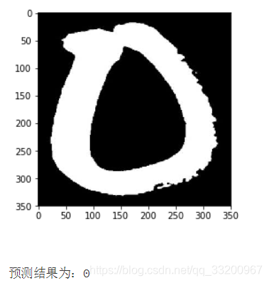
Convert the output result, output the label with the maximum probability, and output the currently predicted image.
lab = np.argsort(result)
im = Image.open('./TibetanMnist(350x350)/0_10_398.jpg')
plt.imshow(im)
plt.show()

print('Prediction result: %d' % lab[0][0][-1])
References
- https://www.kesci.com/home/dataset/5bfe734a95