Mean (Average)
- Represents the central tendency of a set of data and the overall average level.
- The commonly mentioned “zero-centered” or “mean-subtraction” involves subtracting the mean from each value.
\[\mu=\frac{1}{N}\sum_{i=1}^Nx_i\quad(x:x_1,x_2,\ldots,x_N)\]
import numpy as np

# 1D array
x = np.array([-0.02964322, -0.11363636, 0.39417967, -0.06916996, 0.14260276])
print('Data:', x)

# Calculate mean
avg = np.mean(x)
print('Mean:', avg)
Output:
Data: [-0.02964322 -0.11363636  0.39417967 -0.06916996  0.14260276]
Mean: 0.064866578
Standard Deviation
- Represents the dispersion of data in distribution.
- Variance is the square of the standard deviation.
\[\sigma=\sqrt{\frac{1}{N}\sum_{i=1}^N\left(x_i-\mu\right)^2}\quad(x:x_1,x_2,\ldots,x_N)\]
import numpy as np

# 1D array
x = np.array([-0.02964322, -0.11363636, 0.39417967, -0.06916996, 0.14260276])
print('Data:', x)

# Calculate standard deviation
std = np.std(x)
print('Standard Deviation:', std)
Output:
Data: [-0.02964322 -0.11363636  0.39417967 -0.06916996  0.14260276]
Standard Deviation: 0.18614576055671836
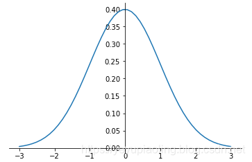
Normal Distribution
- Also called “Gaussian distribution”, one of the most important distributions.
- Mean determines the position, variance determines the amplitude.
- Notation: \(X\sim N\left(\mu,\sigma^2\right)\)
Probability density function of normal distribution:
\(\(f(x)=\frac{1}{\sqrt {2\pi\sigma}}e^{-\frac{\left(x-\mu\right)^2}{2\sigma^2}}\)\)
import numpy as np
from matplotlib import pyplot as plt

def normal_dist(x, mu=0, sigma=1):
    return 1/(np.sqrt(2*np.pi*sigma**2)) * np.exp(-(x - mu)**2/(2*sigma**2))

x = np.linspace(-3, 3, 50)
y = normal_dist(x)
plt.plot(x, y)

# Adjust coordinate system
ax = plt.gca()
ax.spines['right'].set_color('none')
ax.spines['top'].set_color('none')
ax.xaxis.set_ticks_position('bottom')
ax.yaxis.set_ticks_position('left')
ax.spines['bottom'].set_position(('data', 0))
ax.spines['left'].set_position(('data', 0))
plt.show()
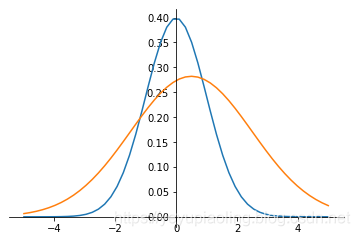
Normalization of Non-Standard Normal Distribution
- Converts non-standard normal distribution to standard normal.
- Formula: Subtract mean and divide by standard deviation for each data point.
\[y=\frac{x-\mu}{\sigma}\]
import numpy as np
from matplotlib import pyplot as plt

def normal_dist(x, mu=0, sigma=1):
    return 1/(np.sqrt(2*np.pi*sigma**2)) * np.exp(-(x - mu)**2/(2*sigma**2))

x = np.linspace(-5, 5, 50)
y1 = normal_dist(x)
y2 = normal_dist(x, mu=0.5, sigma=2)
plt.plot(x, y1)
plt.plot(x, y2)

# Adjust coordinate system
ax = plt.gca()
ax.spines['right'].set_color('none')
ax.spines['top'].set_color('none')
ax.xaxis.set_ticks_position('bottom')
ax.yaxis.set_ticks_position('left')
ax.spines['bottom'].set_position(('data', 0))
ax.spines['left'].set_position(('data', 0))
plt.show()
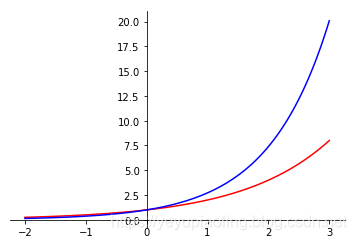
Exponential Function
- Common bases: 2 and e.
- Domain: All real numbers.
- Range: Non-negative numbers.
\[y_1=2^x$$
$$y_2=e^x\]
import numpy as np
from matplotlib import pyplot as plt

x = np.linspace(-2, 3, 100)
y1 = 2**x
y2 = np.exp(x)
plt.plot(x, y1, color='red')
plt.plot(x, y2, color='blue')

# Adjust coordinate system
ax = plt.gca()
ax.spines['right'].set_color('none')
ax.spines['top'].set_color('none')
ax.xaxis.set_ticks_position('bottom')
ax.yaxis.set_ticks_position('left')
ax.spines['bottom'].set_position(('data', 0))
ax.spines['left'].set_position(('data', 0))
plt.show()
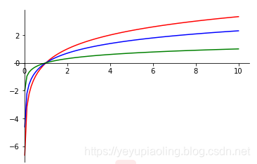
Logarithmic Function
- Common bases: 2, e, 10.
- Domain: Positive numbers.
- Range: All real numbers.
- Output is negative when input is in (0, 1).
\[y_1=\log_2x$$
$$y_2=\ln x$$
$$y_3=\lg x\]
import numpy as np
from matplotlib import pyplot as plt

x = np.linspace(0.01, 10, 100)
y1 = np.log2(x)
y2 = np.log(x)
y3 = np.log10(x)
plt.plot(x, y1, color='red')
plt.plot(x, y2, color='blue')
plt.plot(x, y3, color='green')

# Adjust coordinate system
ax = plt.gca()
ax.spines['right'].set_color('none')
ax.spines['top'].set_color('none')
ax.xaxis.set_ticks_position('bottom')
ax.yaxis.set_ticks_position('left')
ax.spines['bottom'].set_position(('data', 0))
ax.spines['left'].set_position(('data', 0))
plt.show()
Softmax Function
- Activation function in output layer of classification networks, outputting probabilities.
- Steps: Apply exponential function to all outputs, then normalize by dividing by the sum of exponentials.
\[P_i=\frac{e^{x_i}}{\sum_{i=1}^Ne^{x_i}}\quad(x:x_1,x_2,\ldots,x_N)\]
import numpy as np

x = np.array([-0.02964322, -0.11363636, 0.39417967, -0.06916996, 0.14260276])
print('Original Outputs:', x)
prob = np.exp(x) / np.sum(np.exp(x))
print('Probability Outputs:', prob)
Output:
Original Outputs: [-0.02964322 -0.11363636  0.39417967 -0.06916996  0.14260276]
Probability Outputs: [0.17868493 0.16428964 0.27299323 0.17175986 0.21227234]
One-hot Encoding
- Used for class encoding in classification networks.
- Encoding length equals the number of classes.
- Exactly one element is 1, others are 0 in each vector.
- All encoding vectors are orthogonal.
Example:
For 5 classes:
Class 1: [1, 0, 0, 0, 0]
Class 2: [0, 1, 0, 0, 0]
Class 3: [0, 0, 1, 0, 0]
Class 4: [0, 0, 0, 1, 0]
Class 5: [0, 0, 0, 0, 1]
Cross Entropy
- Loss function for classification problems.
- Measures the difference between predicted probability distribution and label distribution.
Label (after one-hot encoding): \([l_1, l_2, \ldots, l_N]\)
Prediction (after Softmax): \([P_1, P_2, \ldots, P_N]\)
\[ce=-\sum_{i=1}^Nl_i\cdot\log(P_i)\]
import numpy as np

# One-hot encoded label
label = np.array([0, 0, 1, 0, 0])
print('Class Label:', label)
# Network outputs
x1 = np.array([-0.02964322, -0.11363636, 3.39417967, -0.06916996, 0.14260276])
x2 = np.array([-0.02964322, -0.11363636, 1.39417967, -0.06916996, 5.14260276])
print('Network Output 1:', x1)
print('Network Output 2:', x2)
# Softmax probabilities
p1 = np.exp(x1) / np.sum(np.exp(x1))
p2 = np.exp(x2) / np.sum(np.exp(x2))
print('Probability Output 1:', p1)
print('Probability Output 2:', p2)
# Cross Entropy
ce1 = -np.sum(label * np.log(p1))
ce2 = -np.sum(label * np.log(p2))
print('Cross Entropy 1:', ce1)
print('Cross Entropy 2:', ce2)
Output:
Class Label: [0 0 1 0 0]
Network Output 1: [-0.02964322 -0.11363636  3.39417967 -0.06916996  0.14260276]
Network Output 2: [-0.02964322 -0.11363636  1.39417967 -0.06916996  5.14260276]
Probability Output 1: [0.02877271 0.02645471 0.88293386 0.0276576  0.03418112]
Probability Output 2: [0.00545423 0.00501482 0.02265122 0.00524284 0.96163688]
Cross Entropy 1: 0.12450498821197674
Cross Entropy 2: 3.787541448750617
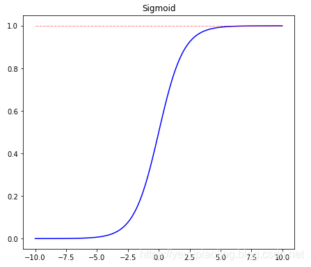
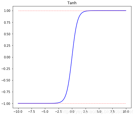
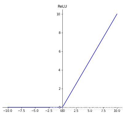
Activation Functions
- Introduce non-linearity to enable powerful model representation.
- Sigmoid and Tanh have saturation regions causing vanishing gradients.
- ReLU and its variants are most commonly used in deep learning.
\[\text{Sigmoid}(x)=\frac{1}{1+e^{-x}}$$
$$\text{Tanh}(x)=\frac{e^x-e^{-x}}{e^x+e^{-x}}$$
$$\text{ReLU}(x)=\max(x, 0)\]
import numpy as np
from matplotlib import pyplot as plt

x = np.linspace(-10, 10, 100)
plt.figure(figsize=(10, 20))

# Sigmoid
sigmoid = 1 / (1 + np.exp(-x))
plt.subplot(311)
plt.plot(x, sigmoid, color='blue')
plt.title('Sigmoid')

# Tanh
tanh = (np.exp(x) - np.exp(-x)) / (np.exp(x) + np.exp(-x))
plt.subplot(312)
plt.plot(x, tanh, color='blue')
plt.title('Tanh')

# ReLU
relu = np.maximum(x, 0)
plt.subplot(313)
plt.plot(x, relu, color='blue')
plt.title('ReLU')

# Adjust coordinate system
ax = plt.gca()
ax.spines['right'].set_color('none')
ax.spines['top'].set_color('none')
ax.xaxis.set_ticks_position('bottom')
ax.yaxis.set_ticks_position('left')
ax.spines['bottom'].set_position(('data', 0))
ax.spines['left'].set_position(('data', 0))
plt.show()
Source Code: https://aistudio.baidu.com/aistudio/projectdetail/176057