Preface¶

In computer vision, stereo vision using a binocular camera is a common approach, with algorithms like BM (Block Matching) and SGBM (Semi-Global Block Matching) being widely used. Unlike laser ranging, binocular ranging does not require a laser light source, making it eye-safe. It only needs cameras, resulting in very low cost, and is applied in most projects. In this chapter, we will introduce how to implement distance measurement using a binocular camera and the SGBM algorithm.

Camera Calibration¶

Each binocular camera is different; factors like their distance and distortion cause differences in their positioning algorithm parameters. Therefore, we typically use camera calibration to obtain these algorithm parameters. The purpose of calibration is to eliminate distortion and obtain internal and external parameter matrices. The internal parameter matrix is related to the focal length and can be understood as a transformation from a plane to pixels. Since the focal length remains constant, it can be reused once determined. The external parameter matrix reflects the transformation between the camera coordinate system and the world coordinate system. Distortion parameters are generally included in the internal parameter matrix. Functionally, the internal parameter matrix captures lens information and eliminates distortion to produce more accurate images, while the external parameter matrix establishes the camera’s relationship with the world coordinate system for final distance measurement.

Capturing Calibration Images¶

We need to capture calibration images using the camera, resulting in images from the left and right eyes. Typically, around 16 images are captured. Binocular cameras usually output left-eye images first, followed by right-eye images. Using OpenCV, we can capture these images and separate them by cropping. The following Python code captures calibration images, saving them when the Enter key is pressed. Note that the camera focus should be adjusted before capturing and not changed afterward:

import cv2

imageWidth = 1280
imageHeight = 720

cap = cv2.VideoCapture(0)
cap.set(cv2.CAP_PROP_FRAME_WIDTH, imageWidth * 2)
cap.set(cv2.CAP_PROP_FRAME_HEIGHT, imageHeight)
i = 0

while True:
    success, img = cap.read()
    if success:
        rgbImageL = img[:, 0:imageWidth, :]
        rgbImageR = img[:, imageWidth:imageWidth * 2, :]
        cv2.imshow('Left', rgbImageL)
        cv2.imshow('Right', rgbImageR)
        c = cv2.waitKey(1) & 0xff
        if c == 13:
            cv2.imwrite('Left%d.bmp' % i, rgbImageL)
            cv2.imwrite('Right%d.bmp' % i, rgbImageR)
            print("Saved image %d" % i)
            i += 1

cap.release()

The following image shows the checkerboard required for calibration. Print it on A3 paper, fix it with a wooden board (avoid bending), and preferably use a professional checkerboard. The checkerboard in the camera’s view should occupy more than one-third of the frame.

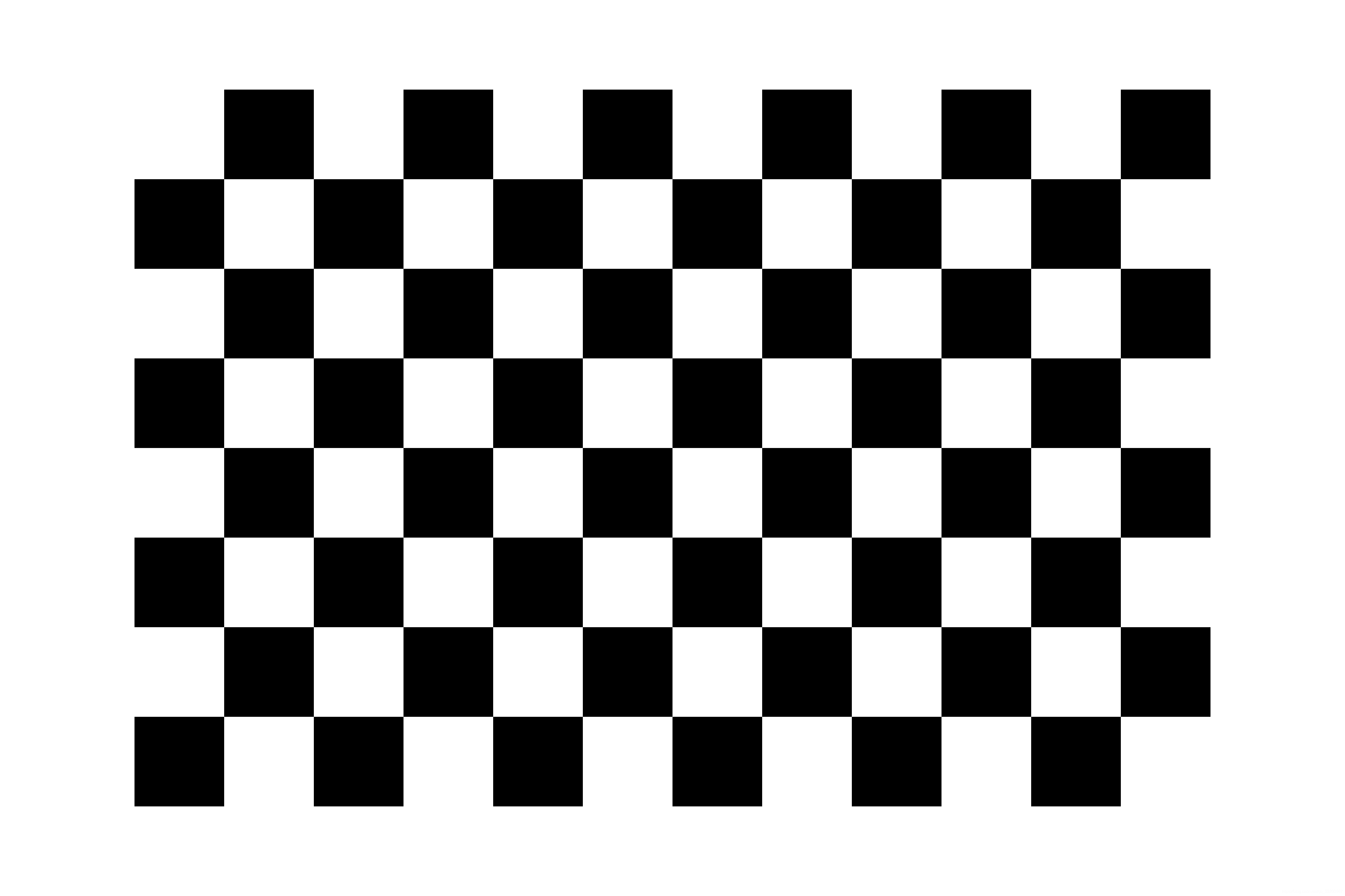
Image Calibration¶

After capturing the images, use MATLAB for calibration. The author used MATLAB R2016a, but other versions should also work.

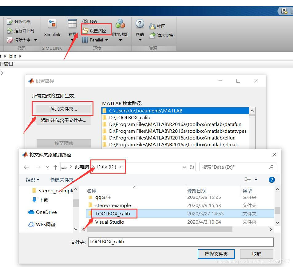
Open MATLAB R2016a, add the path to TOOLBOX_calib. Download TOOLBOX_calib from https://resource.doiduoyi.com/#w0w0sko, extract it to the root directory of drive D, as shown in the image:

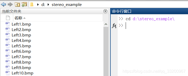
In MATLAB’s command window, enter: cd d:\calib_example to open the folder with calibration images (adjust the path as needed).

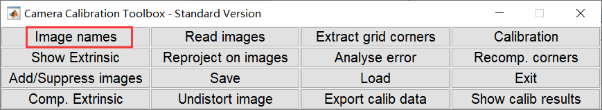
Next, enter: calib_gui in the command window to start the calibration tool, as shown:

Click the Standard(all the images are stored in memory) button. Then a new interface will appear; click Image names to list the calibration images by their names:

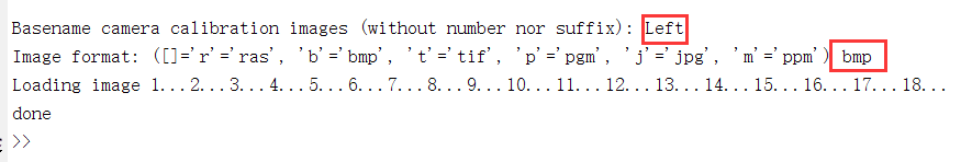
Click Image names to display all images in the current directory. Since the image names vary only by the trailing number, we can specify the prefix as Left and the suffix as bmp to load all left-eye images:

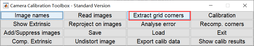
After loading, a window with the left-eye images will appear. Return to the calibration tool interface and click Extract grid corners to start calibration:

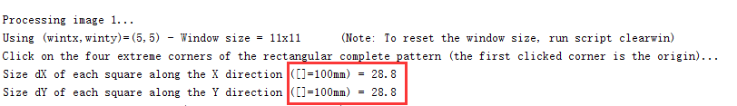
In the command window, press Enter to accept default settings. Two parameters need adjustment based on the checkerboard grid size (e.g., 28.8mm per grid for A3 paper).

After calibration, each image will display corner markers. If the image is undistorted, press Enter to proceed to the next image. For distorted images, adjust parameters (range [-1, 1]) until all markers align with grid corners.

After processing all images, click Calibration in the tool interface to generate calibration results. Save the results as Calib_Results.mat, then rename it to Calib_Results_left.mat for the left eye and Calib_Results_right.mat for the right eye.

Run stereo_gui in the command window, load both calibration files, and click Run stereo calibration to optimize parameters. The output will include focal lengths, principal points, rotation/translation vectors, and disparity parameters for the left and right eyes:

Focal Length (Left): fc_left = [ 781.69191 781.93358 ]
Principal Point (Left): cc_left = [ 319.50000 239.50000 ]
Distortion Coefficients (Left): kc_left = [ 0.02704 0.10758 -0.00408 -0.01769 0.00000 ]
Rotation Vector (om): om = [ -0.01044 -0.04553 -0.00143 ]
Translation Vector (T): T = [ -60.87137 0.15622 0.01502 ] (baseline distance)

Distance Measurement¶

This chapter uses the SGBM algorithm, a global matching algorithm with better performance than local methods but higher complexity. SGBM is available in OpenCV via cv2.StereoSGBM_create.

The following Python code implements binocular ranging using pre-calibrated parameters and SGBM:

import cv2
import numpy as np

imageWidth = 1280
imageHeight = 720
imageSize = (imageWidth, imageHeight)

# Left-eye camera calibration parameters
cameraMatrixL = np.array([[849.38718, 0, 720.28472],
                          [0, 850.60613, 373.88887],
                          [0, 0, 1]])
distCoeffL = np.array([0.01053, 0.02881, 0.00144, 0.00192, 0.00000])

# Right-eye camera calibration parameters
cameraMatrixR = np.array([[847.54814, 0, 664.36648],
                          [0, 847.75828, 368.46946],
                          [0, 0, 1]])
distCoeffR = np.array([0.00905, 0.02094, 0.00082, 0.00183, 0.00000])

# Extrinsic parameters
R = cv2.Rodrigues(np.array([-0.00927, -0.00228, -0.00070]))[0]
T = np.array([-59.32102, 0.27563, -0.79807])

Stereo Rectification & SGBM Setup:

# Rectify images
mapLx, mapLy = cv2.initUndistortRectifyMap(cameraMatrixL, distCoeffL, R, 
                                           cv2.stereoRectify(cameraMatrixL, distCoeffL, 
                                                             cameraMatrixR, distCoeffR, 
                                                             imageSize, R, T)[3], 
                                           imageSize, cv2.CV_32FC1)
mapRx, mapRy = cv2.initUndistortRectifyMap(cameraMatrixR, distCoeffR, R, 
                                           cv2.stereoRectify(...)[4], imageSize, cv2.CV_32FC1)

# Read images
rectifyImageL = cv2.remap(cv2.cvtColor(cv2.imread("Left3.bmp"), cv2.COLOR_BGR2GRAY), 
                          mapLx, mapLy, cv2.INTER_LINEAR)
rectifyImageR = cv2.remap(cv2.cvtColor(cv2.imread("Right3.bmp"), cv2.COLOR_BGR2GRAY), 
                          mapRx, mapRy, cv2.INTER_LINEAR)

# SGBM parameters
sgbm = cv2.StereoSGBM_create(minDisparity=32, numDisparities=176, blockSize=16)
sgbm.setP1(4 * 1 * 16 * 16)
sgbm.setP2(32 * 1 * 16 * 16)

disp = sgbm.compute(rectifyImageL, rectifyImageR)

# 3D reconstruction
xyz = cv2.reprojectImageTo3D(disp, cv2.reprojectImageTo3D(...), handleMissingValues=True)
xyz = xyz * 16  # Scale factor

Visualization & Mouse Callback:

# Normalize disparity map for visualization
disp8U = cv2.normalize(disp.astype(np.float32)/16, None, 0, 255, cv2.NORM_MINMAX, dtype=cv2.CV_8U)

def onMouse(event, x, y, flags, param):
    if event == cv2.EVENT_LBUTTONDOWN:
        print(f"Point ({x}, {y}): 3D Coordinates {xyz[y, x]}")

cv2.imshow("Disparity", disp8U)
cv2.setMouseCallback("Disparity", onMouse)
cv2.waitKey(0)
cv2.destroyAllWindows()

Output Example:

Point (777, 331): 3D Coordinates [57.85, -23.24, 519.85]
Point (553, 383): 3D Coordinates [-70.19, 6.37, 525.83]

The black regions in the disparity map indicate unmeasurable distances or objects too far.

Source Code Download: Download Here